A customer recently asked if IRIS supported OpenTelemetry as they where seeking to measure the time that IRIS implemented SOAP Services take to complete. The customer already has several other technologies that support OpenTelemetry for process tracing.  At this time, InterSystems IRIS (IRIS) do not natively support OpenTelemetry.  

Is there a difference in outcome between the two screengrabs below?

In both cases, when  certain conditions are met, a transformation is called and the output sent on to two targets. In the first case we surmise the transformation is called twice, and the output of the first run sent to the first target, the output of the second run to the second target. In the second case we surmise the transformation is called once, and the output duplicated and sent to the two targets. 

So if you are following from the previous post or dropping in now, let's segway to the world of eBPF applications and take a look at Parca, which builds on our brief investigation of performance bottlenecks using eBPF, but puts a killer app on top of your cluster to monitor all your iris workloads, continually, cluster wide!  

Continous Profiling with Parca, IRIS Workloads Cluster Wide

I attended Cloud Native Security Con in Seattle with full intention of crushing OTEL day, then perusing the subject of security applied to Cloud Native workloads the following days leading up to CTF as a professional excercise. This was happily upended by a new understanding of eBPF, which got my screens, career, workloads, and atitude a much needed upgrade with new approaches to solving workload problems. 

So I made it to the eBPF party and have been attending clinic after clinic on the subject ever since, here I would like to "unbox" eBPF as a technical solution, mapped directly to what we do in practice (even if its a bit off), and step through eBPF through my experimentation on supporting InterSystems IRIS Workloads, particularly on Kubernetes, but not necessarily void on standalone workloads.

eBee Steps with eBPF and InterSystems IRIS Workloads

Question:can a business process with pool size > 1 invoke external programs in parallel via $ZF(-100)?

We have a production that takes HL7 (ORU_R01) messages in and produces a PDF from each one for onward transmission to a document store.

It's been a long time since I didn't write an update post on IoP.

So what's new since IoP command line interface was released?

Two new big features were added to IoP:

• Rebranding: the grongier.pex module was renamed to iop to reflect the new name of the project.
• Async support: IoP now supports async functions and coroutines.

Rebranding

The grongier.pex module was renamed to iop to reflect the new name of the project.

The grongier.pex module is still available for backward compatibility, but it will be removed in the future.

Async support

IoP supports async calls for a long time, but it was not possible to use async functions and coroutines directly in IoP.

Before jumping into this new feature, I will explain how async calls work in InterSystems IRIS and present two examples of how to use async calls IoP.

Legacy async calls

Let's see how legacy async calls work:

from iop import BusinessProcess
from msg import MyMessage


class MyBP(BusinessProcess):

    def on_message(self, request):
        msg_one = MyMessage(message="Message1")
        msg_two = MyMessage(message="Message2")

        self.send_request_async("Python.MyBO", msg_one,completion_key="1")
        self.send_request_async("Python.MyBO", msg_two,completion_key="2")

    def on_response(self, request, response, call_request, call_response, completion_key):
        if completion_key == "1":
            self.response_one = call_response
        elif completion_key == "2":
            self.response_two = call_response

    def on_complete(self, request, response):
        self.log_info(f"Received response one: {self.response_one.message}")
        self.log_info(f"Received response two: {self.response_two.message}")

Basically they work the same way as async call works in IRIS. The send_request_async method sends a request to a Business Operation and the on_response method is called when the response is received.

You can distinguish the responses by the completion_key parameter.

Send multiple sync requests

It's not exactly a new feature, but it's worth mentioning that you can send multiple sync requests in parallel:

from iop import BusinessProcess
from msg import MyMessage


class MyMultiBP(BusinessProcess):

    def on_message(self, request):
        msg_one = MyMessage(message="Message1")
        msg_two = MyMessage(message="Message2")

        tuple_responses = self.send_multi_request_sync([("Python.MyMultiBO", msg_one),
                                                        ("Python.MyMultiBO", msg_two)])

        self.log_info("All requests have been processed")
        for target,request,response,status in tuple_responses:
            self.log_info(f"Received response: {response.message}")

Here we are sending two requests to the same Business Operation in parallel.

The response is a tuple with the target, request, response and status of each call.

It's really useful when you need to send multiple requests and you don't care about the order of the responses.

Async functions and coroutines

Now let's see how to use async functions and coroutines in IoP:

import asyncio

from iop import BusinessProcess
from msg import MyMessage


class MyAsyncNGBP(BusinessProcess):

    def on_message(self, request):

        results = asyncio.run(self.await_response(request))

        for result in results:
            print(f"Received response: {result.message}")

    async def await_response(self, request):
        msg_one = MyMessage(message="Message1")
        msg_two = MyMessage(message="Message2")

        # use asyncio.gather to send multiple requests asynchronously
        # using the send_request_async_ng method
        tasks = [self.send_request_async_ng("Python.MyAsyncNGBO", msg_one),
                 self.send_request_async_ng("Python.MyAsyncNGBO", msg_two)]

        return await asyncio.gather(*tasks)

In this example, we are sending multiple requests to the same Business Operation in parallel using the send_request_async_ng method.

If you read this post carefully until this point, please comment "Boomerang". This is may be a detail for you, but for me it's mean a lot. Thanks!

The await_response method is a coroutine that sends multiple requests and waits for all responses to be received. Thanks to the asyncio.gather function, we can wait for all responses to be received in parallel.

The benefits of using async functions and coroutines are:

• Better performance: you can send multiple requests in parallel.
• Easier to read and maintain: you can use the await keyword to wait for responses.
• More flexibility: you can use the asyncio module to create complex workflows.
• More control: you can use the asyncio module to handle exceptions and timeouts.

Conclusion

What are the defirences between send_request_async, send_multi_request_sync and send_request_async_ng?

• send_request_async: sends a request to a Business Operation and waits for the response if the on_response method is implemented and the completion_key parameter is used.
  • benefit: you can use async calls the way you are used to.
  • drawback: you can be hard to maintain if you need to send multiple requests in parallel.
• send_multi_request_sync: sends multiple requests to the same Business Operation in parallel and waits for all responses to be received.
  • benefit: it's easy to use.
  • drawback: you can control the order of the responses (i mean the list of responses is not ordered).
• send_request_async_ng: sends multiple requests to the same Business Operation in parallel and waits for all responses to be received.
  • benefit: you can control the order of the responses.
  • drawback: you need to use async functions and coroutines.

Happy multithreading!

When there's a performance issue, whether for all users on the system or a single process, the shortest path to understanding the root cause is usually to understand what the processes in question are spending their time doing.  Are they mostly using CPU to dutifully march through their algorithm (for better or worse); or are they mostly reading database blocks from disk; or mostly waiting for something else, like LOCKs, ECP or database block collisions?

Hi Community, 
We invite you to join our next Meetup in Cambridge, MA on August 28, 5:30-7:30 pm.
>> RSVP here <<
 

Hello Community,

As per the Build index documentation "If you use BUILD INDEX on a live system, the index is temporarily labeled as notselectable, meaning that queries cannot use the index while it is being built. Note that this will impact the performance of queries that use the index." Is this  hiding/not selectable is only applicable for BUILD INDEX or it supports class level %BuildIndices as well. as far as my analysis both syntax setting this setting SetMapSelectability. 

Thanks!

There are often questions surrounding the ideal Apache HTTPD Web Server configuration for HealthShare.  The contents of this article will outline the initial recommended web server configuration for any HealthShare product. 

As a starting point, Apache HTTPD version 2.4.x (64-bit) is recommended.  Earlier versions such as 2.2.x are available, however version 2.2 is not recommended for performance and scalability of HealthShare.

Hello everyone,

Recently, I've been working on a Business Process that processes a large JSON FHIR message containing up to 50k requests in an array within the JSON.

Currently, the code imports the JSON as a dynamic object from the original message stream, obtains an iterator from it, and processes each request one at a time in a loop.

We are experimenting with IIS, as the PWS will be gone in newer versions.

The code which is executed, takes 15ms to run. If we execute it through PWS (REST), there is some overhead and the total execution time is 40ms, which is acceptable. However, if we go through IIS, it takes 150ms or sometimes even more.

Both PWS and IIS are running on the same server as IRIS in this case. No optimisations have been done on IIS.

Any suggestions on where to look/what to optimize on IIS?

[Background]

InterSystems IRIS family has a nice utility ^SystemPerformance (as known as ^pButtons in Caché and Ensemble) which outputs the database performance information into a readable HTML file. When you run ^SystemPerformance on IRIS for Windows, a HTML file is created where both our own performance log mgstat and Windows performance log are included.

You may have heard about our mg-dbx-napi interface for IRIS which provides insanely fast access from Node.js.  If you've been following recent developments in the server-side JavaScript world, you'll be excited to know that mg-dbx-napi also works with Bun.js, the latter proving to be significantly faster than Node.js for many/most purposes.

Of course, if you're a Node.js user, you'll probably wonder how mg-dbx-napi compares with the Native API for Node.js that is included with IRIS.

With all that in mind, we've created a Github repository: mg-showcase

Online document says: TUNE TABLE updates the SQL table definition (and therefore requires privileges to alter the table definition). Commonly, TUNE TABLE also updates the corresponding persistent class definition. This allows the gathered statistics to be used by the query optimizer without requiring a class compilation.

It seems like yesterday when we did a small project in Java to test the performance of IRIS, PostgreSQL and MySQL (you can review the article we wrote back in June at the end of this article). If you remember, IRIS was superior to PostgreSQL and clearly superior to MySQL in insertions, with no big difference in queries.

Well, shortly after @Dmitry Maslennikov told me "Why don't you test it from a Python project?" Well, here is the Python version of the tests we previously performed using the JDBC connections.

Windows Subsystem for Linux (WSL) is a feature of Windows that allows you to run a Linux environment on your Windows machine, without the need for a separate virtual machine or dual booting. 

WSL is designed to provide a seamless and productive experience for developers who want to use both Windows and Linux at the same time**.

Most transactional applications have a 70:30 RW profile. However, some special cases have extremely high write IO profiles.

I ran storage IO tests in the ap-southeast-2 (Sydney) AWS region to simulate IRIS database IO patterns and throughput similar to a very high write rate application.

The test aimed to determine whether the EC2 instance types and EBS volume types available in the AWS Australian regions will support the high IO rates and throughput required.

Minimal tuning was done in the operating system or IRIS (see Operating System and IRIS configuration below).

• The EC2 instance and EBS volume types were selected to maximise IOPS and throughput.

The following tests were run:

• Using a single io2 Block Express volumes each for database and WIJ.
• Using a Logical Volume Manager (LVM) striped volume of 16 gp3 disks for the database and a five gp3 disk LVM striped volume for the WIJ.
• Two instances in separate availability zones using IRIS synchronous database mirroring using a single io2 Block Express volume for the database and WIJ on each instance.

Summary

A limited number of tests were run. However, the results show that running a high IO rate IRIS workload in the Sydney AWS region is possible.

There are limits everywhere in the cloud

• It is worth noting that along with the published IOPS and throughput limits for instances and storage, AWS has limits at the account level. AWS was required to lift InterSystems account regional default IOPS quotas to enable testing at high IO rates—specifically, EBS - IOPS for Provisioned IOPS SSD (io2) volumes to 600,000.
  • Remember to review limits before starting its tests, especially mirroring tests, as all volumes in the region are included in the same total.

EBS Volume Types

• IO Tests were run with the IRIS database using a single EBS io2 Block Express volume and multiple (16) EBS gp3 volumes using Logical Volume Manager (LVM).
  • The database write IOPS, throughput, and latency were similar between the io2 Block Express and gp3 LVM tests. Database write latency was around 1 ms.
  • The read latency of gp3 was two times io2 Block Express. However, the gp3 maximum read latency was still acceptable at less than 0.8 ms.
  • WIJ write latency was around 50% higher on a single io2 Block Express volume than on a five-volume gp3 LVM stripe.
  • For details on io2 Block Express, see https://aws.amazon.com/ebs/provisioned-iops/.
  • For details on gp3, see https://aws.amazon.com/ebs/general-purpose/.

EC2 Instance Types

• At the time of testing in July 2023, only one EC2 memory-optimised instance type (r5b) in the Sydney region uses the nitro system capable of running io2 Block Express volumes.
  • The EC2 instance type selected must be capable of matching or exceeding the storage IO and throughput needed for the data and WIJ volumes.
  • The only instance types in Sydney supporting the io2 Block Express are r5b and c7g. c7g was not used due to lower IOPS and low memory.
  • io2 Block Express is required for higher throughput and IOPS (256,000 IOPS per volume) compared to standard io2 (64,000 IOPS per volume).
  • EC2 instances capable of using io2 Block Express are not currently available in Melbourne.

The Tests

• The publicly available RANREAD and RANWRITE utilities were used to simulate the IRIS IO profile. For example, RANWRITE uses the IRIS WD cycle, resulting in a burst of large WIJ IOs and random database writes that are not usually expected or understood by storage vendors.
  • For an overview of LVM, RANREAD, and RANWRITE utilities, see https://community.intersystems.com/post/using-lvm-stripe-increase-aws-ebs-iops-and-throughput.
  • At higher IOPS and throughput, the overall results and IO profile are not expected to change; for example, there will be a longer WD cycle at peak storage IOPS at the observed latency.

AWS Environment

The following environment was tested in ap-southeast-2 (Sydney). The same instance type was used for all tests for an apples-to-apples comparison.

EC2 instance profile

EC2 instance type: 

• R5b.24xlarge: 96 vCPU, 780 GB Memory, 25 Gbps network.
  • EBS limits per EC2 instance: 
    • Maximum throughput (MB/s) 7,500
    • Maximum IOPS 260,000

The benchmark suite uses a 4MB LVM stripe whether there are single or multiple volumes. All volumes use the xfs filesystem.

Benchmark tests

• For test 1 and test 2, the WIJ is on a separate volume.
  • The WIJ and database could be on the same volume to save on storage costs.
  • However, having the WIJ on a separate volume isolates the impact of the WIJ on database reads.
  • The journal volume is always separate from the WIJ and database volumes.

Test 1 - io2 Block Express

Storage layout

• Journal
  • Single gp3 volume. I used the defaults: 3,000 IOPS and 125 MB/s throughput.
• WIJ
  • Single io2 Block Express volume. 256,000 IOPS and 4,000 MB/s throughput.
• Database
  • Single io2 Block Express volume. 100,000 IOPS and 4,000 MB/s throughput.

Test 2 - gp3 LVM stripe

Storage layout

• Journal
  • Single gp3 volume. I used the defaults: 3,000 IOPS and 125 MB/s throughput.
• WIJ
  • Five gp3 volumes. Each 16,000 IOPS and 1,000 MB/s throughput. Total 80,000 IOPS and 5,000 MB/s throughput.
• Database
  • 16 gp3 volumes. Each 16,000 IOPS and 1,000 MB/s throughput. Total 256,000 IOPS and 16,000 MB/s throughput.

Test 3 - IRIS asynchronous database mirror - io2 Block Express

A database mirror was created with the primary mirror member in AWS availability zone b and the backup mirror member in availability zone c. The arbiter was in availability zone a.

• The same read/write IO rate was run as the other tests.

Storage layout

• Due to the total 600,000 IOPS quota across all volumes, the WIJ and database are on the same io2 Block Express volume. Allowing a total of (256K + 256K) 512 IOPS across the mirrors.

• Journal

  • Single gp3 volume. I used the defaults: 3,000 IOPS and 125 MB/s throughput.

• WIJ and Database

  • Single io2 Block Express volume. 256,000 IOPS and 4,000 MB/s throughput.

Observations

Database Read IO

The chart below shows io2 Block Express has approximately half the latency as an LVM stripe of gp3 volumes. The benchmark tests are paced using a set number of processes, with the result you get half the IOPS at twice the latency. An application-based test may provide different results, or the pace of the tests could be changed to increase the processes and resulting IOPS.

Database Write IO

The chart below shows similar peak IOPS and latency between io2 Block Express and an LVM stripe of gp3 volumes. The higher write latency of the Primary mirror database is because the WIJ is on the same volume, the higher latency is the WIJ, the random database writes latency was similar to io2 Block Express. Latency is measured for non-zero writes.

WIJ Write IO

The chart below shows higher throughput for an LVM stripe of gp3 volumes. However, this is misleading, as the io2 Block Express volume had higher throughput and a shorter WIJ write time. Further investigation may show, for example, larger IOs on the io2 Block Express volume. Latency is measured for non-zero writes.

Throughput

Throughput is one of the metrics AWS charges for and is a metric that has a maximum per EC2 instance (10,000 MB/s) and per EBS volume (4,000 MB/s for io2 Block Express and 1,000 MB/s for gp3). Similar to the way IOPS are monitored and throttled by AWS by increasing latency. The following chart shows the kB/s throughput. The throughput requirements must be known to ensure that under-provisioning throughput does not become a bottleneck. The WIJ throughput is higher than the provisioned throughput per volume; this can happen as AWS takes a few seconds to register that higher than provisioned IOPS or throughput is occurring before limiting.

Database writes impact on database read latency.

The charts show the trends. However, many details will come out by examining the metrics more closely. For example, database reads are impacted by a burst of writes on the same volume. The larger-sized writes of the WIJ have a more significant impact. The io patterns of the different volume types are interesting as well.

io2 Block Express

The following chart shows the stepped increases in the read process during the io2 Block Express test. Note the dip in reads when the storage has to read and write simultaneously.

The following chart shows the corresponding spikes in latency. Note the smooth read IOPS in the chart above and the flat latency below.

gp3 LVM stripe

The same charts for the LVM stripe of gp3 disks show the less stable io pattern (sometimes called jitter) of gp3 disks.

Compare the baseline read latency to the maximum latency for the different volume types.

Other details

IRIS Configuration

The IRIS version test was 2023.2.0.204.0

Minimal configuration was done for IRIS. A snippet of the cpf file is shown below.

[config]
Asyncwij=16
:
globals=0,0,589824,0,0,0
:
wdparm=16,32,512,128
wduseasyncio=1

• Asyncwij = 16 means 16 in flight, WIJ writes at a time. The default is eight.

The wdparm parameter is used to configure the number of slave write daemons, the size of the device ID table (used for assigning writes to WDs), the maximum number of outstanding writes across all WDs, and whether or not the database will adjust the number of allowed writes PER WD if some WDs are inactive or finish early on a given pass.

16 = Number of write daemons (8 is the default)
32 = Size of the device ID table (32 is the default)
512 = Max number of outstanding IOs for all write daemons
128 = Max number of outstanding IOs per write daemon

AWS AZ ping times on the day of the mirror test

The Primary mirror was in AZ b; the backup mirror was in AZ c.

• Ping AZ b to AZ c average 1.16ms
• Ping AZ c to AZ b average 1.12ms

Hi Community,

Watch this video to learn how InterSystems software enables both horizontal and vertical scaling:

⏯ Scaling for User and Data Volume in InterSystems IRIS

InterSystems IRIS offers various ways how to profile your code, in most cases it produces enough information to find the places where the most time is spent or where the most global sets. But sometimes it's difficult to understand the execution flow and how it ended at that point. 

To solve this, I've decided to implement a way to build a report in a way, so, it's possible to dive by stack down

Hello,

I would like to get a list of all globals that have been read or written during a given context. In Portal, there are counters in dashboard that give the number of read/write to globals in general.

What I am looking for : 

- some handler (eg: like $ZTRAP) that will be called everytime something is read/written to a global.

- to activate a "global log mode" in Portal that will dump some information to a file (like ^ISCSOAP for SOAP requests).

I understand this is something that can considerably slow down IRIS, but it's intended to be used only for debbuging and under no load.

I am often asked to review customers' IRIS application performance data to understand if system resources are under or over-provisioned.

This recent example is interesting because it involves an application that has done a "lift and shift" migration of a large IRIS database application to the Cloud. AWS, in this case.

A key takeaway is that once you move to the Cloud, resources can be right-sized over time as needed. You do not have to buy and provision on-premises infrastructure for many years in the future that you expect to grow into.

Continuous monitoring is required. Your application transaction rate will change as your business changes, the application use or the application itself changes. This will change the system resource requirements. Planners should also consider seasonal peaks in activity. Of course, an advantage of the Cloud is resources can be scaled up or down as needed.

For more background information, there are several in-depth posts on AWS and IRIS in the community. A search for "AWS reference" is an excellent place to start. I have also added some helpful links at the end of this post.

AWS services are like Lego blocks, different sizes and shapes can be combined. I have ignored networking, security, and standing up a VPC for this post. I have focused on two of the Lego block components;

• Compute requirements.
• Storage requirements.

Overview

The application is a healthcare information system used at a busy hospital group. The architecture components I am focusing on here include two database servers in an InterSystems mirror failover cluster.

Sidebar: Mirrors are in separate availability zones for additional high availability.

Compute requirements

EC2 Instance Types

Amazon EC2 provides a wide selection of instance types optimised for different use cases. Instance types comprise varying FIXED combinations of CPU and memory and fixed upper limits on storage and networking capacity. Each instance type includes one or more instance sizes.

EC2 instance attributes to look at closely include:

• vCPU cores and Memory.
• Maximum IOPS and IO throughput.

For IRIS applications like this one with a large database server, two types of EC2 instances are a good fit: 

• EC2 R5 and R6i are in the Memory Optimised family of instances and are an ideal fit for memory-intensive workloads, such as IRIS. There is 8GB memory per vCPU.
• EC2 M5 and M6i are in the General Purpose family of instances. There is 4GB memory per vCPU. They are used more for web servers, print servers and non-production servers.

Note: Not all instance types are available in all AWS regions. R5 instances were used in this case because the more recently released R6i was unavailable.

Capacity Planning

When an existing on-premises system is available, capacity planning means measuring current resource use, translating that to public cloud resources, and adding resources for expected short-term growth. Generally, if there are no other resource constraints, IRIS database applications scale linearly on the same processors; for example, imagine adding a new hospital to the group; increasing system use (transaction rate) by 20% will require 20% more vCPU resources using the same processor types. Of course, that's not guaranteed; validate your applications.

vCPU requirements

Before the migration, CPU utilisation peaked near 100% at busy times; the on-premises server has 26 vCPUs. A good rule of thumb is to size systems with an expected peak of 80% CPU utilisation. This allows for transient spikes in activity or other unusual activity. An example CPU utilisation chart for a typical day is shown below.

Monitoring the on-premises servers would prompt an increase in vCPUs to 30 cores to bring general peak utilisation below 80%. The customer was anticipating adding 20% transaction growth in the short term. So, a 20% buffer is added to the calculations, also allowing some extra headroom for the migration period.

A simple calculation is that 30 cores + 20% growth and migration buffer is 36 vCPU cores required. 

Sizing for the cloud

Remember, AWS EC2 instances in each family type come in fixed sizes of vCPU and memory and set upper limits on IOPS, storage, and network throughput.

For example, available instance types in the R5 and R6i families include:

• 16 vCPUs and 128GB memory
• 32 vCPUs and 256 GB memory
• 48 vCPUs and 384 GB memory
• 64 vCPUs and 512 GB memory
• And so on.

Rule of thumb: A simplified way to size an EC2 instance from known on-premises metrics to the cloud is to round up the recommended on-premises vCPU requirements to the next available EC2 instance size.

Caveats: There can be many other considerations; for example, differences in on-premises and EC2 processor types and speeds, or having more performant storage in the cloud than an old on-premises system, can mean that vCPU requirements change, for example, more IO and more work can be done in less time, increasing peak vCPU utilisation. On-premises servers may have a full CPU processor, including hyper-threading, while cloud instance vCPUs are a single hyper thread. On the other hand, EC2 instances are optimised to offload some processing to onboard Nitro cards allowing the main vCPU cores to spend more cycles processing workloads, thus delivering better instance performance. But, in summary, the above rule is a good guide to start. The advantage of the cloud is that with continuous monitoring, you can plan and change the instance type to optimise performance and cost.

For example, to translate 30 or 36 vCPUs on-premises to similar EC2 instance types:

• The r5.8xlarge has 32 vCPUs, 256 GB memory and a maximum of 30,000 IOPS.
• The r512xlarge has 48 vCPUs, 384 GB memory and a maximum of 40,000 IOPS

Note the maximum IOPS. This will become important later in the story.

Results

An r512xlarge instance was selected for the IRIS database mirrors for the migration.

In the weeks after migration, monitoring showed the 48 vCPU instance type with sustained peaks near 100% vCPU utilisation. Generally, though, the processing peaked at around 70%. Well within the acceptable range, and if the periods of high utilisation can be traced to a process that can be optimised, there is plenty of headroom to consider right-sizing to a lower specification and cheaper EC2 instance type.

Sometime later, the instance type remained the same. A system performance check shows that the general peak vCPU utilisation has dropped to around 50%. However, there are still transient peaks near 100%.

Recommendation

Continuous monitoring is required. With constant monitoring, the system can be right-sized to achieve the necessary performance and be cheaper to run.

The transient spikes in vCPU utilisation should be investigated. For example, a report or batch job may be moved out of business hours, lowering the overall vCPU peak and lessening any adverse impact on interactive application users.

Review the storage IOPS and throughput requirements before changing the instance type; remember, instance types have fixed limits on maximum IOPS.

Instances can be right-sized by using failover mirroring. Simplified steps are:

• Power off the backup mirror.
• Power on the backup mirror using a smaller or larger instance with configuration changes to mount the EBS storage and account for a smaller memory footprint (think about things like Linux hugepages and IRIS global buffers).
• Let the backup mirror catch up.
• Failover the backup mirror to become primary.
• Repeat, resize the remaining mirror, return it online, and catch up.

Note: During the mirror failover, there will be a short outage for all users, interfaces, etc. However, if ECP application servers are used, there can be no interruption to users. Application servers can also be part of an autoscaling solution.

Other cost-saving options include running the backup mirror on a smaller instance. However, there is a significant risk of reduced performance (and unhappy users) if a failover occurs at peak processing times.

Caveats: Instance vCPU and memory are fixed. Restarting with a smaller instance with a smaller memory footprint will mean a smaller global buffer cache, which can increase the database read IOPS. Please take into account the storage requirements before reducing the instance size. Automate and test rightsizing to minimise the risk of human error, especially if it is a common occurrence.

Storage requirements

Predictable storage IO performance with low latency is vital to provide scalability and reliability for your applications.

Storage types

Amazon Elastic Block Store (EBS) storage is recommended for most high transaction rate IRIS database applications. EBS provides multiple volume types that allow you to optimise storage performance and cost for a broad range of applications. SSD-backed storage is required for transactional workloads such as applications using IRIS databases.

Of the SSD storage types, gp3 volumes are generally recommended for IRIS databases to balance price and performance for transactional applications; however, for exceptional cases with very high IOPS or throughput, io2 can be used (typically for a higher cost). There are other options, such as locally attached ephemeral storage and third-party virtual array solutions. If you have requirements beyond io2 capabilities, talk to InterSystems about your needs.

Storage comes with limits and costs, for example;

• gp3 volumes deliver a baseline performance of 3,000 IOPS and 125 MiBps at any volume size with single-digit millisecond latency 99% of the time for the base cost of the storage GB capacity. gp3 volumes can scale up to 16,000 IOPS and 1,000 MiBps throughput for an additional cost. Storage is priced per GB and on provisioned IOPS over the 3,000 IOPS baseline.
• io2 volumes deliver a consistent baseline performance of up to 500 IOPS/GB to a maximum of 64,000 IOPS with single-digit millisecond latency 99.9% of the time. Storage is priced per GB and on provisioned IOPS.

Remember: EC2 instances also have limits on total EBS IOPS and throughput. For example, the r5.8xlarge has 32 vCPUs and a maximum of 30,000 IOPS. Not all instance types are optimised to use EBS volumes.

Capacity Planning

When an existing on-premises system is available, capacity planning means measuring current resource use, translating that to public cloud resources, and adding resources for expected short-term growth.

The two essential resources to consider are:

• Storage capacity. How many GB of database storage do you need, and what is the expected growth? For example, you know your on-premises system's historical average database growth for a known transaction rate. In that case, you can calculate future database sizes based on any anticipated transaction rate growth. You will also need to consider other storage, such as journals.
• IOPS and throughput. This is the most interesting and is covered in detail below.

Database requirements

Before the migration, database disk reads were peaking at around 8,000 IOPS.

Read plus Write IOPS was peaking above 40,000 on some days. Although, during business hours, the peaks are much lower.

The total throughput of reads plus writes was peaking at around 600 MB/s.

Remember, EC2 instances and EBS volumes have limits on IOPS AND throughput. Whichever limit is reached first will result in the throttling of that resource by AWS, causing performance degradation and likely impacting the users of your system. You must provision IOPS AND throughput.

Sizing for the cloud

For a balance of price and performance, gp3 volumes are used. However, in this case, the limit of 16,000 IOPS for a single gp3 volume is exceeded, and there is an expectation that requirements will increase in the future.

To allow for the provisioning of higher IOPS than is possible on a single gp3 volume, an LVM stripe is used.

For the migration, the database is deployed using an LVM stripe of four gp3 volumes with the following:

• Provisioned 8,000 IOPS on each volume (for a total of 32,000 IOPS).
• Provisioned throughput of 250 MB/s on each volume (for a total of 1,000 MB/s).

The exact capacity planning process was done for the Write Image Journal (WIJ) and transaction journal on-premises disks. The WIJ and journal disks were each provisoned on a single gp3 disk.

For more details and an example of using an LVM stripe, see: https://community.intersystems.com/post/using-lvm-stripe-increase-aws-ebs-iops-and-throughput

Rule of thumb: If your requirements exceed the limits of a single gp3 volume, investigate the cost difference between using LVM gp3 and io2 provisioned IOPS.

Caveats: Ensure the EC2 instance does not limit IOPS or throughput.

Results

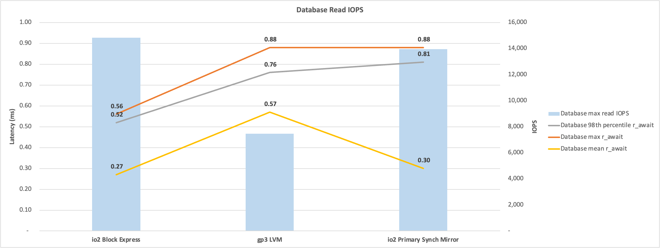
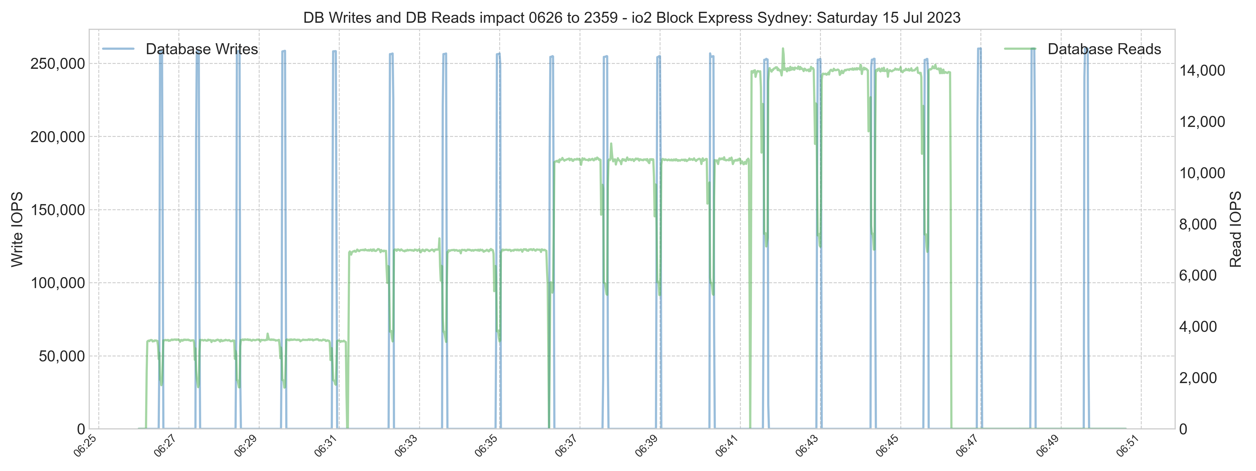
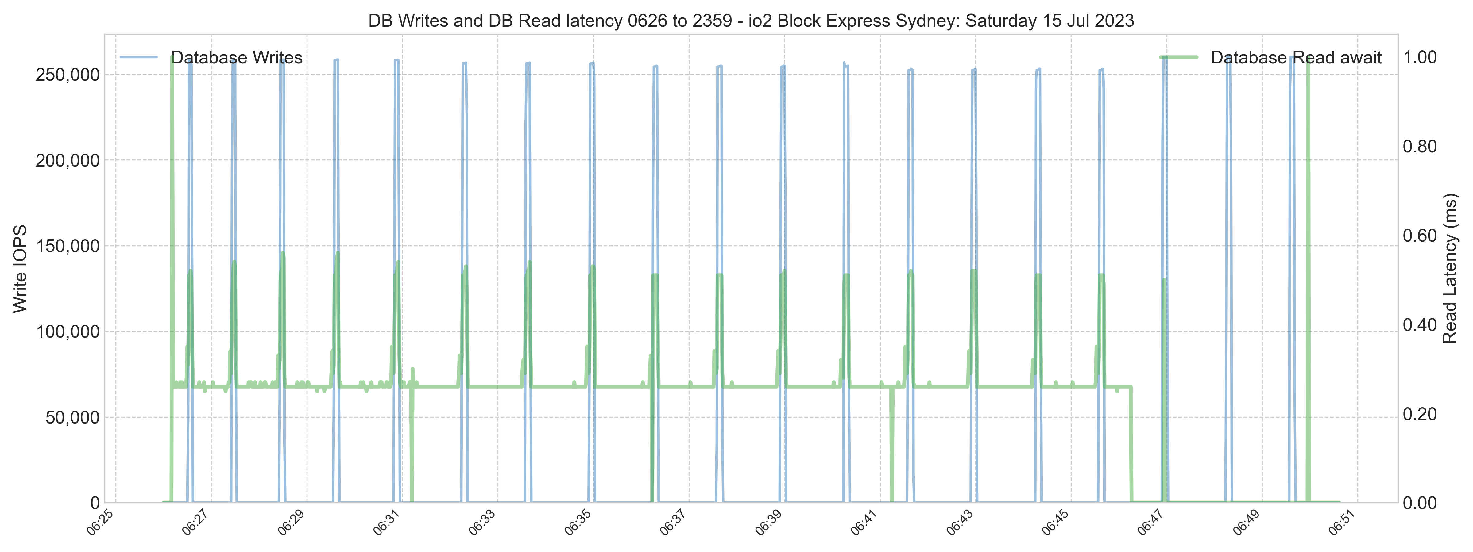
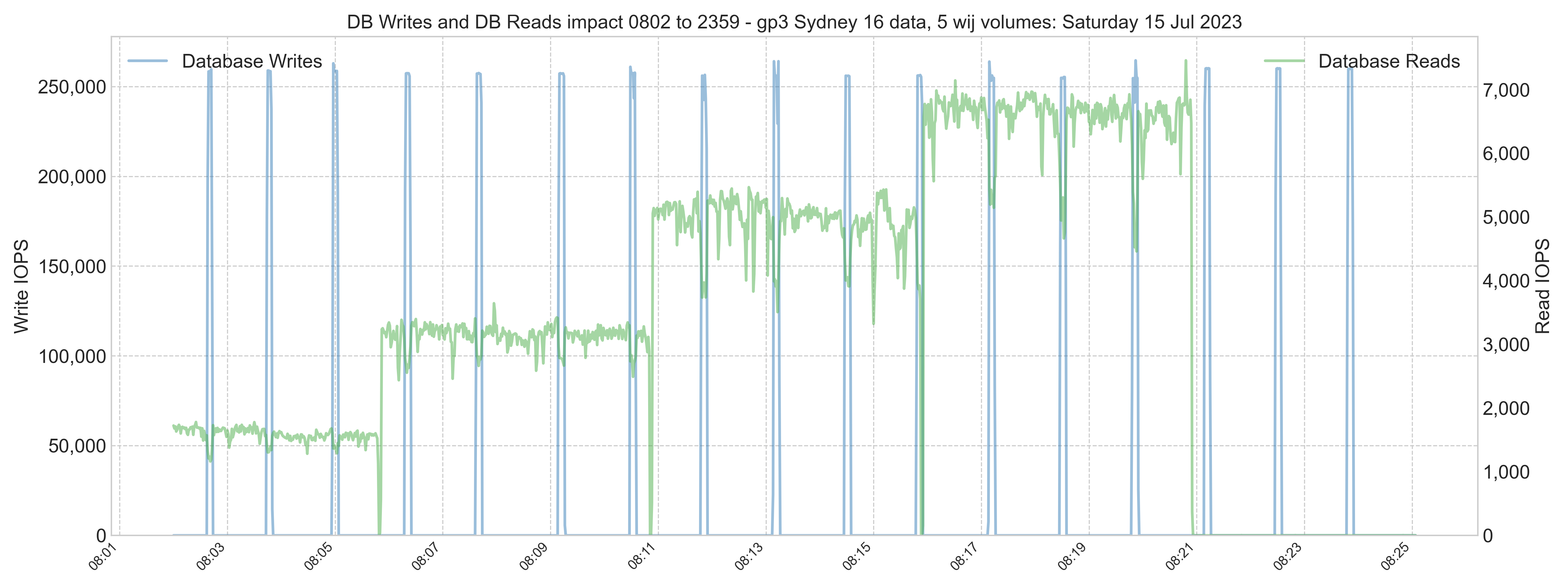
In the weeks after migration, database write IOPS peaked at around 40,000 IOPS, similar to on-premises. However, the database reads IOPS were much lower.

Lower read IOPS is expected due to the EC2 instance having more memory available for caching data in global buffers. More application working set data in memory means it does not have to be called in from much slower SSD storage. Remember, the opposite will happen if you reduce the memory footprint.

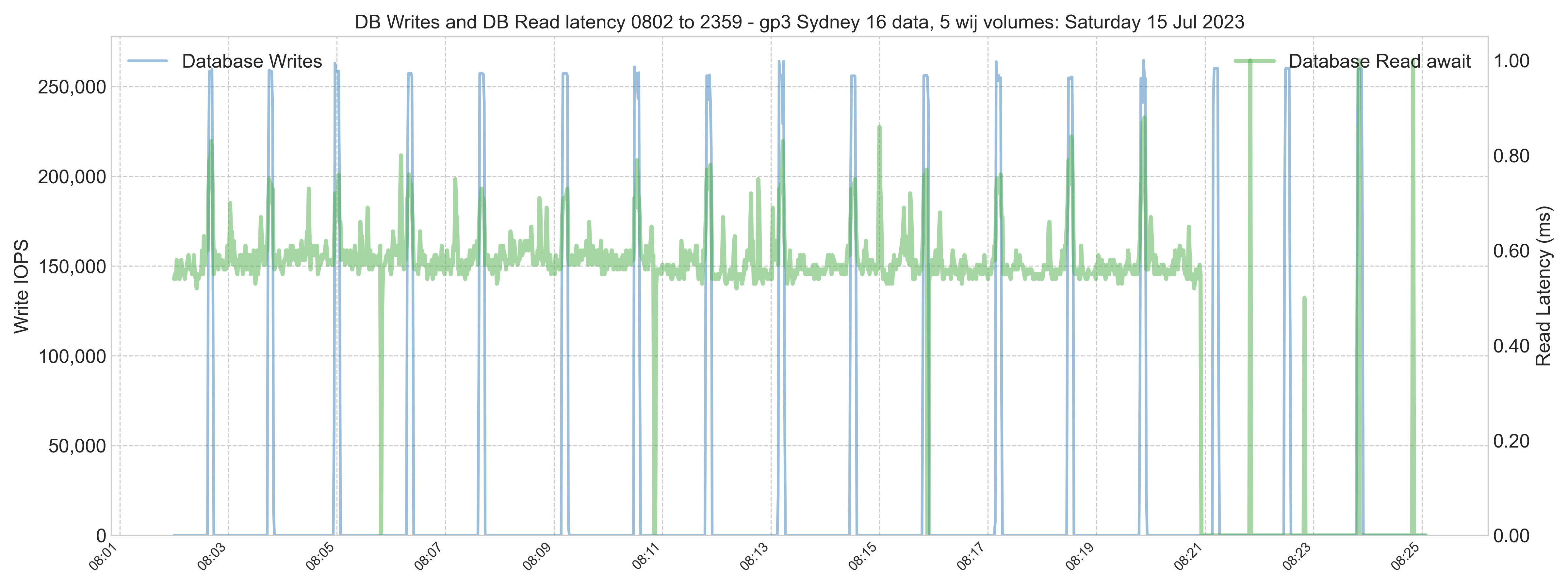
During peak processing times, the database volume had spikes above 1 ms latency. However, the spikes are transient and will not impact the user's experience. Storage performance is excellent.

Later, a system performance check shows that although there are some peaks, generally, read IOPS is still lower than on-premises.

Recommendation

Continuous monitoring is required. With constant monitoring, the system can be right-sized to achieve the necessary performance and be cheaper to run.

An application process responsible for the 20 minutes of high overnight database write IOPS (chart not shown) should be reviewed to understand what it is doing. Writes are not affected by large global buffers and are still in the 30-40,000 IOPS range. The process could be completed with lower IOPS provisioning. However, there will be a measurable impact on database read latency if the writes overwhelm the IO path, adversely affecting interactive users. Read latency must be monitored closely if reads are throttled for an extended period.

The database disk IOPS and throughput provisioning can be adjusted via AWS APIs or interactively via the AWS console. Because four EBS volumes comprise the LVM disk, the IOPS and throughput attributes of the EBS volumes must be adjusted equally.

The WIJ and journal should also be continuously monitored to understand if any changes can be made to the IOPS and throughput provisioning.

Note: The WIJ volume has high throughput requirements (not IOPS) due to the 256 kB block size. WIJ volume IOPS may be under the baseline of 3,000 IOPS, but throughput is currently above the throughput baseline of 125 MB/s. Additional throughput is provisioned in the WIJ volume.

Caveats: Decreasing IOPS provisioning to throttle the period of high overnight writes will result in a longer write daemon cycle (WIJ plus random database writes). This may be acceptable if the writes finish within 30-40 seconds. However, there may be a severe impact on read IOPS and read latency and, therefore, the experience of interactive users on the system for 20 minutes or longer. Please be sure to proceed with caution.

Helpful links

• Charts are created with "yaspe" https://community.intersystems.com/post/yaspe-yet-another-system-performance-extractor

AWS

• Details of AWS Elastic Cloud Computing (EC2) can be found here: https://aws.amazon.com/ec2/
• Details of AWS Elastic Block Store (EBS) can be found here: https://aws.amazon.com/ebs/

I deployed the IRIS container on my Mac M1 Docker Desktop Kubernetes cluster:

I limited the container 1.5Gb memory:

In the "merge.cpf" file I constrained IRIS memory usage aspects:

Now I load-test the container by multiple installing  and uninstalling the %ZPM package:

• install ZPM (zpm-installer.routine and execution):

Hey Developers,

Enjoy watching the new video on InterSystems Developers YouTube:

⏯ System Performance Review for InterSystems IRIS Applications @ Global Summit 2022

Hi guys,

I'm working on a project with my client.
They have a visit table which has about 7,000,000 records. The table is used in a random search page witch holds 20+ conditions to be combined.
The table is defined as below:

A good writer is supposed to draw you in with the title and bury the answer somewhere in the article.  I suppose this makes me a bad writer – don’t think less of me, my whole feeling of self-worth comes from the opinions of internet strangers! 

In terms of general through-put design and long term support, I'm considering what would be a "best approach" for needing to create multiple batch files in a few different layouts from the same data-sets.

YASPE is the successor to YAPE (Yet Another pButtons Extractor). YASPE has been written from the ground up with many internal changes to allow easier maintenance and enhancements.

YASPE functions:

• Parse and chart InterSystems Caché pButtons and InterSystems IRIS SystemPerformance files for quick performance analysis of Operating System and IRIS metrics.
• Allow a deeper dive by creating ad-hoc charts and by creating charts combining the Operating System and IRIS metrics with the "Pretty Performance" option.
• The "System Overview" option saves you from searching your SystemPerformance files for system details or common configuration options.

YASPE is written in Python and is available on GitHub as source code or for Docker containers at:

• https://github.com/murrayo/yaspe

YASPE is more focused on the current Operating System and IRIS versions. If you run older versions and have problems with YASPE, you can see if you successfully run your performance files through YAPE. If you have problems, do not hesitate to contact me through GitHub.

Examples

Output files

Options include:

• HTML or PNG charts for all columns in mgstat and vmstat or windows perfmon and output to folders.
• It is optional to create charts for iostat as this can take a long time if there is a big disk list.
• A CSV file for further manual processing, for example, with Excel.

Pretty Performance

Below is the example custom chart, Glorefs (mgstat) and Total CPU utilisation (vmstat).

Below is one of the default images, which includes a zoom to a specified time (or defaults to 13:00-14:00).

System Overview

yaspe includes a system overview and basic config check (-s)

This check is designed to save you from hunting through your SystemPerformance file looking for system details. An example of overview.txt follows:

System Summary for your site name

Hostname         : YOURHOST
Instance         : SHADOW
Operating system : Linux
Platform         : N/A
CPUs             : 24
Processor model  : Intel(R) Xeon(R) Gold 6248 CPU @ 2.50GHz
Memory           : 126 GB
Shared memory    : globals 71680 MB + routines 1023 MB + gmheap 1000 MB = 73,703 MB
Version          : Cache for UNIX (Red Hat Enterprise Linux for x86-64) 2018.1.4 (Build 505_1U) Thu May 28 2020 10:11:16 EDT
Date collected   : Profile run "24hours" started at 16:15:00 on Nov 22 2021.

Warnings:
- Journal freeze on error is not enabled. If journal IO errors occur database activity that occurs during this period cannot be restored.
- swappiness is 10. For databases 5 is recommended to adjust how aggressive the Linux kernel swaps memory pages to disk.
- Hugepages not set. For performance, memory efficiency and to protect the shared memory from paging out, use huge page memory space. It is not advisable to specify HugePages much higher than the shared memory amount because the unused memory are not be available to other components.
- dirty_background_ratio is 10. InterSystems recommends setting this parameter to 5. This setting is the maximum percentage of active memory that can be filled with dirty pages before pdflush begins to write them.
- dirty_ratio is 30. InterSystems recommends setting this parameter to 10. This setting is the maximum percentage of total memory that can be filled with dirty pages before processes are forced to write dirty buffers themselves during their time slice instead of being allowed to do more writes. These changes force the Linux pdflush daemon to write out dirty pages more often rather than queue large amounts of updates that can potentially flood the storage with a large burst of updates

Recommendations:
- Review and fix warnings above
- Set HugePages, see IRIS documentation: https://docs.intersystems.com/irislatest/csp/docbook/Doc.View.cls?KEY=GCI_prepare_install#GCI_memory_big_linux
- Total memory is 128,755 MB, 75% of total memory is 96,566 MB.
- Shared memory (globals+routines+gmheap) is 73,703 MB. (57% of total memory).
- Number of HugePages for 2048 KB page size for (73,703 MB + 5% buffer = 77,388 MB) is 38694

All instances on this host:
- >SHADOW            2018.1.4.505.1.a  56772  /cachesys

Your application is deployed and everything is running fine. Great, hi-five! Then out of the blue the phone starts to ring off the hook – it’s users complaining that the application is sometimes ‘slow’. But what does that mean? Sometimes? What tools do you have and what statistics should you be looking at to find and resolve this slowness? Is your system infrastructure up to the task of the user load? What infrastructure design questions should you have asked before you went into production? How can you capacity plan for new hardware with confidence and without over-spec'ing? How can you stop the phone ringing? How could you have stopped it ringing in the first place?

InterSystems Data Platforms and performance - Part 5 Monitoring with SNMP

In previous posts I have shown how it is possible to collect historical performance metrics using pButtons. I go to pButtons first because I know it is installed with every Data Platforms instance (Ensemble, Caché, …). However there are other ways to collect, process and display Caché performance metrics in real time either for simple monitoring or more importantly for much more sophisticated operational analytics and capacity planning. One of the most common methods of data collection is to use SNMP (Simple Network Management Protocol).

SNMP a standard way for Caché to provide management and monitoring information to a wide variety of management tools. The Caché online documentation includes details of the interface between Caché and SNMP. While SNMP should 'just work' with Caché there are some configuration tricks and traps. It took me quite a few false starts and help from other folks here at InterSystems to get Caché to talk to the Operating System SNMP master agent, so I have written this post so you can avoid the same pain.

In this post I will walk through the set up and configuration of SNMP for Caché on Red Hat Linux, you should be able to use the same steps for other *nix flavours. I am writing the post using Red Hat because Linux can be a little more tricky to set up - on Windows Caché automatically installs a DLL to connect with the standard Windows SNMP service so should be easier to configure.

Once SNMP is set up on the server side you can start monitoring using any number of tools. I will show monitoring using the popular PRTG tool but there are many others - Here is a partial list.

Note the Caché and Ensemble MIB files are included in the Caché_installation_directory/SNMP folder, the file are: ISC-CACHE.mib and ISC-ENSEMBLE.mib.

Previous posts in this series:

• Part 1 - Getting started on the Journey, collecting metrics.
• Part 2 - Looking at the metrics we collected.
• Part 3 - Focus on CPU.
• Part 4 - Looking at memory.

Start here...

Start by reviewing Monitoring Caché Using SNMP in the Caché online documentation.

1. Caché configuration

Follow the steps in Managing SNMP in Caché section in the Caché online documentation to enable the Caché monitoring service and configure the Caché SNMP subagent to start automatically at Caché startup.

Check that the Caché process is running, for example look on the process list or at the OS:

ps -ef | grep SNMP
root      1171  1097  0 02:26 pts/1    00:00:00 grep SNMP
root     27833     1  0 00:34 pts/0    00:00:05 cache -s/db/trak/hs2015/mgr -cj -p33 JOB^SNMP

Thats all, Caché configuration is done!

2. Operating system configuration

There is a little more to do here. First check that the snmpd daemon is installed and running. If not then install and start snmpd.

Check snmpd status with:

service snmpd status

Start or Stop snmpd with:

service snmpd start|stop

If snmp is not installed then you will have to install as per OS instructions, for example:

yum -y install net-snmp net-snmp-utils

3. Configure snmpd

As detailed in the Caché documentation, on Linux systems the most important task is to verify that the SNMP master agent on the system is compatible with the Agent Extensibility (AgentX) protocol (Caché runs as a subagent) and the master is active and listening for connections on the standard AgentX TCP port 705.

This is where I ran into problems. I made some basic errors in the snmp.conf file that meant the Caché SNMP subagent was not communicating with the OS master agent. The following sample /etc/snmp/snmp.conf file has been configured to start agentX and provide access to the Caché and ensemble SNMP MIBs.

Note you will have to confirm whether the following configuration complies with your organisations security policies.

At a minimum the following lines must be edited to reflect your system set up.

For example change:

syslocation  "System_Location"

to

syslocation  "Primary Server Room"

Also edit the at least the following two lines:

syscontact  "Your Name"
trapsink  Caché_database_server_name_or_ip_address public 	

Edit or replace the existing /etc/snmp/snmp.conf file to match the following:

###############################################################################
#
# snmpd.conf:
#   An example configuration file for configuring the NET-SNMP agent with Cache.
#
#   This has been used successfully on Red Hat Enterprise Linux and running
#   the snmpd daemon in the foreground with the following command:
#
#	/usr/sbin/snmpd -f -L -x TCP:localhost:705 -c./snmpd.conf
#
#   You may want/need to change some of the information, especially the
#   IP address of the trap receiver of you expect to get traps. I've also seen
#   one case (on AIX) where we had to use  the "-C" option on the snmpd command
#   line, to make sure we were getting the correct snmpd.conf file. 
#
###############################################################################

###########################################################################
# SECTION: System Information Setup
#
#   This section defines some of the information reported in
#   the "system" mib group in the mibII tree.

# syslocation: The [typically physical] location of the system.
#   Note that setting this value here means that when trying to
#   perform an snmp SET operation to the sysLocation.0 variable will make
#   the agent return the "notWritable" error code.  IE, including
#   this token in the snmpd.conf file will disable write access to
#   the variable.
#   arguments:  location_string

syslocation  "System Location"

# syscontact: The contact information for the administrator
#   Note that setting this value here means that when trying to
#   perform an snmp SET operation to the sysContact.0 variable will make
#   the agent return the "notWritable" error code.  IE, including
#   this token in the snmpd.conf file will disable write access to
#   the variable.
#   arguments:  contact_string

syscontact  "Your Name"

# sysservices: The proper value for the sysServices object.
#   arguments:  sysservices_number

sysservices 76

###########################################################################
# SECTION: Agent Operating Mode
#
#   This section defines how the agent will operate when it
#   is running.

# master: Should the agent operate as a master agent or not.
#   Currently, the only supported master agent type for this token
#   is "agentx".
#   
#   arguments: (on|yes|agentx|all|off|no)

master agentx
agentXSocket tcp:localhost:705

###########################################################################
# SECTION: Trap Destinations
#
#   Here we define who the agent will send traps to.

# trapsink: A SNMPv1 trap receiver
#   arguments: host [community] [portnum]

trapsink  Caché_database_server_name_or_ip_address public 	

###############################################################################
# Access Control
###############################################################################

# As shipped, the snmpd demon will only respond to queries on the
# system mib group until this file is replaced or modified for
# security purposes.  Examples are shown below about how to increase the
# level of access.
#
# By far, the most common question I get about the agent is "why won't
# it work?", when really it should be "how do I configure the agent to
# allow me to access it?"
#
# By default, the agent responds to the "public" community for read
# only access, if run out of the box without any configuration file in 
# place.  The following examples show you other ways of configuring
# the agent so that you can change the community names, and give
# yourself write access to the mib tree as well.
#
# For more information, read the FAQ as well as the snmpd.conf(5)
# manual page.
#
####
# First, map the community name "public" into a "security name"

#       sec.name  source          community
com2sec notConfigUser  default       public

####
# Second, map the security name into a group name:

#       groupName      securityModel securityName
group   notConfigGroup v1           notConfigUser
group   notConfigGroup v2c           notConfigUser

####
# Third, create a view for us to let the group have rights to:

# Make at least  snmpwalk -v 1 localhost -c public system fast again.
#       name           incl/excl     subtree         mask(optional)
# access to 'internet' subtree
view    systemview    included   .1.3.6.1

# access to Cache MIBs Caché and Ensemble
view    systemview    included   .1.3.6.1.4.1.16563.1
view    systemview    included   .1.3.6.1.4.1.16563.2
####
# Finally, grant the group read-only access to the systemview view.

#       group          context sec.model sec.level prefix read   write  notif
access  notConfigGroup ""      any       noauth    exact  systemview none none

After editing the /etc/snmp/snmp.conf file restart the snmpd deamon.

service snmpd restart

Check the snmpd status, note that AgentX has been started see the status line: Turning on AgentX master support.

h-4.2# service snmpd restart
Redirecting to /bin/systemctl restart  snmpd.service
sh-4.2# service snmpd status
Redirecting to /bin/systemctl status  snmpd.service
● snmpd.service - Simple Network Management Protocol (SNMP) Daemon.
   Loaded: loaded (/usr/lib/systemd/system/snmpd.service; disabled; vendor preset: disabled)
   Active: active (running) since Wed 2016-04-27 00:31:36 EDT; 7s ago
 Main PID: 27820 (snmpd)
   CGroup: /system.slice/snmpd.service
		   └─27820 /usr/sbin/snmpd -LS0-6d -f

Apr 27 00:31:36 vsan-tc-db2.iscinternal.com systemd[1]: Starting Simple Network Management Protocol (SNMP) Daemon....
Apr 27 00:31:36 vsan-tc-db2.iscinternal.com snmpd[27820]: Turning on AgentX master support.
Apr 27 00:31:36 vsan-tc-db2.iscinternal.com snmpd[27820]: NET-SNMP version 5.7.2
Apr 27 00:31:36 vsan-tc-db2.iscinternal.com systemd[1]: Started Simple Network Management Protocol (SNMP) Daemon..
sh-4.2# 

After restarting snmpd you must restart the Caché SNMP subagent using the ^SNMP routine:

%SYS>do stop^SNMP()

%SYS>do start^SNMP(705,20)

The operating system snmpd daemon and Caché subagent should now be running and accessible.

4. Testing MIB access

MIB access can be checked from the command line with the following commands. snmpget returns a single value:

snmpget -mAll -v 2c -c public vsan-tc-db2 .1.3.6.1.4.1.16563.1.1.1.1.5.5.72.50.48.49.53

SNMPv2-SMI::enterprises.16563.1.1.1.1.5.5.72.50.48.49.53 = STRING: "Cache for UNIX (Red Hat Enterprise Linux for x86-64) 2015.2.1 (Build 705U) Mon Aug 31 2015 16:53:38 EDT"

And snmpwalk will 'walk' the MIB tree or branch:

snmpwalk -m ALL -v 2c -c public vsan-tc-db2 .1.3.6.1.4.1.16563.1.1.1.1

SNMPv2-SMI::enterprises.16563.1.1.1.1.2.5.72.50.48.49.53 = STRING: "H2015"
SNMPv2-SMI::enterprises.16563.1.1.1.1.3.5.72.50.48.49.53 = STRING: "/db/trak/hs2015/cache.cpf"
SNMPv2-SMI::enterprises.16563.1.1.1.1.4.5.72.50.48.49.53 = STRING: "/db/trak/hs2015/mgr/"
etc
etc

There are also several windows and *nix clients available for viewing system data. I use the free iReasoning MIB Browser. You will have to load the ISC-CACHE.MIB file into the client so it knows the structure of the MIB.

The following image shows the iReasoning MIB Browser on OSX.

Including in Monitoring tools

This is where there can be wide differences in implementation. The choice of monitoring or analytics tool I will leave up to you.

Please leave comments to the post detailing the tools and value you get from them for monitoring and managing your systems. This will be a big help for other community members.

Below is a screen shot from the popular PRTG Network Monitor showing Caché metrics. The steps to include Caché metrics in PRTG are similar to other tools.

Example workflow - adding Caché MIB to monitoring tool.

Step 1.

Make sure you can connect to the operating system MIBs. A tip is to do your trouble-shooting against the operating system not Caché. It is most likely that monitoring tools already know about and are preconfigured for common operating system MIBs so help form vendors or other users may be easier.

Depending on the monitoring tool you choose you may have to add an SNMP 'module' or 'application', these are generally free or open source. I found the vendor instructions pretty straight forward for this step.

Once you are monitoring the operating system metrics its time to add Caché.

Step 2.

Import the ISC-CACHE.mib and ISC-ENSEMBLE.mib into the tool so that it knows the MIB structure.

The steps here will vary; for example PRTG has a 'MIB Importer' utility. The basic steps are to open the text file ISC-CACHE.mib in the tool and import it to the tools internal format. For example Splunk uses a Python format, etc.

Note: I found the PRTG tool timed out if I tried to add a sensor with all the Caché MIB branches. I assume it was walking the whole tree and timed out for some metrics like process lists, I did not spend time troubleshooting this, instead I worked around this problem by only importing the performance branch (cachePerfTab) from the ISC-CACHE.mib.

Once imported/converted the MIB can be reused to collect data from other servers in your network. The above graphic shows PRTG using Sensor Factory sensor to combine multiple sensors into one chart.

Summary

There are many monitoring, alerting and some very smart analytics tools available, some free, others with licences for support and many and varied functionality.

You must monitor your system and understand what activity is normal, and what activity falls outside normal and must be investigated. SNMP is a simple way to expose Caché and Ensemble metrics.