#InterSystems Business Solutions and Architectures

0 Followers · 90 Posts

This topic unites publications, which describe business ideas and approaches, success stories, architectures, and demos of solutions you can create, build, and implement with InterSystems products: InterSystems IRIS, InterSystems IRIS for Health, HealthShare, Caché, and Ensemble. 

InterSystems staff + admins Hide everywhere
Hidden post for admin
Article Yuri Marx · Jun 22, 2020 1m read

The Intersystems IRIS is a great platform to develop, run and consume Data Science services. IRIS can ingest data from any type, format, protocol and time using adapters. These datasets can be prepared with BPL, DTL and Object Script and stored as SQL or NoSQL data. Finally, it can be consumed by open ML algorithms inside IRIS and visualized in the IRIS dashboards. See more in:   https://docs.intersystems.com/irislatest/csp/docbook/Doc.View.cls?KEY=PAGE_data_science.

0
2 311
Article Yuri Marx · Jun 17, 2020 1m read

In 2017, Forbes published an article talking about API Economy (see: https://www.forbes.com/sites/louiscolumbus/2017/01/29/2017-is-quickly-b…). This article was the trigger to popularize the use of API and API Management by large companies. The article published a maturity model. My understanding is that Intersystems IRIS allows you to reach the top of the pyramid with your current technologies. See the figure above.For this it is important to combine % CSP.REST package, IRIS API Manager (IAM), ML Pack and IntegratedML, Native API for Python, BPL and

0
2 562
Article Yuri Marx · Jun 8, 2020 3m read

About regulations

Personal data privacy regulations have become an indispensable requirement for projects dealing with personal data. The compliance with these laws is based on 4 principles:

  1. Compliance with the rights of the holder of personal data;
  2. Governance of personal data assets;
  3. Privacy by Design and by Default;
  4. Data protection.

In case of violation in the treatment of personal data, controllers and operators of these data may suffer:

0
2 445
Article Murray Oldfield · Apr 1, 2016 2m read

Previously I showed you how to run pButtons to start collecting performance metrics that we are looking at in this series of posts.


##Update: May 2020.

Since this post was written several years ago, we have moved from Caché to IRIS. See the comments for an updated link to the documentation for pButtons (Caché) and SystemPerformance (IRIS). Also, a note on how to update your systems to the latest versions of the performance tools.


pButtons is compatible with Caché version 5 and later and is included with recent distributions of InterSystems data platforms (HealthShare, Ensemble and Caché). This post reminds you that you should download and install the latest version of pButttons.

The latest version is always available for download:

Update:See the comments below for details

To check which version you have installed now, you can run the following:

%SYS>write $$version^pButtons()

Note 1:

  • The current version of pButtons will require a license unit; future distributions will address this requirement.
  • With this distribution of pButtons, versioning has changed. — The prior version of pButtons was 1.16c — This new distribution is version 5.

Note 2:

  • pButtons version 5 also corrects a problem introduced with version 1.16a that could result in prolonged collection times. Version 1.16a was included with Caché 2015.1.0. If you have pButtons version 1.16a through 1.16c, you should download pButtons version 5 from the FTP site.

More detailed information on pButtons is available in the files included with the download and in the online Caché documentation.

2
0 1693
Article Mark Bolinsky · Mar 3, 2020 11m read

InterSystems and Intel recently conducted a series of benchmarks combining InterSystems IRIS with 2nd Generation Intel® Xeon® Scalable Processors, also known as “Cascade Lake”, and Intel® Optane™ DC Persistent Memory (DCPMM). The goals of these benchmarks are to demonstrate the performance and scalability capabilities of InterSystems IRIS with Intel’s latest server technologies in various workload settings and server configurations. Along with various benchmark results, three different use-cases of Intel DCPMM with InterSystems IRIS are provided in this report.

5
0 1093
Article Anton Umnikov · Feb 11, 2020 19m read

InterSystems IRIS Deployment Guide for AWS using CloudFormation template 

Please note: following this guide, especially the prerequisites section requires Intermediate to Advanced level of knowledge of AWS. You'll need to create and manage S3 buckets, IAM roles for EC2 instances, VPCs and Subnets. You'll also need access to InterSystems binaries (usually downloaded via WRC site) as well as IRIS license key.
 

Aug 12, 2020
Anton Umnikov

Templates Source code is available here: https://github.com/antonum/AWSIRISDeployment

Table of Contents

InterSystems IRIS Deployment Guide – AWS Partner Network. 1

1
1 1777
Announcement Amir Samary · Jan 29, 2020

Hi everyone,

I am very pleased to announce that the Readmission Demo has been released as open source. Many thanks to the Solution Factory team that worked hard on making this possible.

Here are the changes:

0
2 590
Article Mark Bolinsky · Mar 21, 2017 4m read

Database systems have very specific backup requirements that in enterprise deployments require forethought and planning. For database systems, the operational goal of a backup solution is to create a copy of the data in a state that is equivalent to when application is shut down gracefully.  Application consistent backups meet these requirements and Caché provides a set of APIs that facilitate the integration with external solutions to achieve this level of backup consistency.

7
2 2892
Article Murray Oldfield · Mar 25, 2016 14m read

This week I am going to look at CPU, one of the primary hardware food groups :) A customer asked me to advise on the following scenario; Their production servers are approaching end of life and its time for a hardware refresh. They are also thinking of consolidating servers by virtualising and want to right-size capacity either bare-metal or virtualized. Today we will look at CPU, in later posts I will explain the approach for right-sizing other key food groups - memory and IO.

So the questions are:

  • How do you translate application requirements on a processor from more than five years ago to todays processors?
  • Which of the current processors are suitable?
  • How does virtualization effect CPU capacity planning?

Added June 2017: For a deeper dive into the specifics of VMware CPU considerations and planning and some common questions and problems, please also see this post: Virtualizing large databases - VMware cpu capacity planning


[A list of other posts in this series is here](https://community.intersystems.com/post/capacity-planning-and-performance-series-index)

Comparing CPU performance using spec.org benchmarks

To translate CPU usage between processor types for applications built using InterSystems data platforms (Caché, Ensemble, HealthShare) you can use SPECint benchmarks as a reliable back of the envelope calculator for scaling between processors. The http://www.spec.org web site has trusted results of a standardised set of benchmarks that are run by hardware vendors.

Specifically SPECint is a way to compare processors between processor models from the same vendors and between different vendors (e.g. Dell, HP, Lenovo, and Intel, AMD, IBM POWER and SPARC). You can use SPECint to understand the expected CPU requirements for your application when hardware is to be upgraded or if your application will be deployed on a range of different customer hardware and you need to set a baseline for a sizing metric, for example peak transactions per CPU core for Intel Xeon E5-2680 (or whatever processor you choose).

There are several benchmarks used on the SPECint web site, however the SPECint_rate_base2006 results are the best for Caché and have been confirmed over many years looking at customer data and in our own benchmarks.

As an example in this post we will compare the difference between the customers Dell PowerEdge server running Intel Xeon 5570 processors and a current Dell server running Intel Xeon E5-2680 V3 processors. The same methodology can be applied when Intel Xeon V4 server processors are generally available (expected soon as I write this in early 2016).

Example: Comparing processors

Search the spec.org database for the SPECint2006_Rates for processor name, for example E5-2680 V3, further refine your search results if your target server make and model is known (e.g Dell R730), otherwise use a popular vendor, I find Dell or HP models are good baselines of a standard server, there is not usually much variance between processors on different vendor hardware.

At the end of this post I walk through a step by step example of searching for results using the spec.org web site…

Lets assume you have searched spec.org and have found the existing server and a possible new server as follows:

Existing: Dell PowerEdge R710 with Xeon 5570 2.93 GHz: 8 cores, 2 chips, 4 cores/chip, 2 threads/core: SPECint_rate_base2006 = 251

New: PowerEdge R730 with Intel Xeon E5-2680 v3, 2.50 GHz: 24 cores, 2 chips, 12 cores/chip, 2 threads/core: SPECint_rate_base2006 = 1030

Not surprisingly the newer 24-core server has more than 4x increase in SPECint_rate_base2006 benchmark throughput of the older 8-core server even though the newer server has a lower clock speed. Note the examples are two-processor servers that have both processor sockets populated.

Why is SPECint_rate_base2006 used for Caché?

The spec.org web site has explanations of the various benchmarks, but the summary is the SPECint_rate2006 benchmark is a complete system-level benchmark uses all CPUs with hyper threading.

Two metrics are reported for a particular SPECint_rate2006 benchmark, base and peak. Base is a conservative benchmark, peak is aggressive. For capacity planning use SPECint_rate_base2006 results.

Does four times the SPECint_rate_base2006 mean four times the capacity for users or transactions?

Its possible that if all 24 cores were used the application throughput could scale to four times the capability of the old server. However several factors can cause this milage to vary. SPECint will get you in the ballpark for sizing and throughput that should be possible, but there are a few caveats.

While SPECint gives a good comparison between the two servers in the example above it is not a guarantee that the E5-2680 V3 server will have 75% more capacity for peak concurrent users or peak transaction throughput as the older Xeon 5570 based server. Other factors come into play such as whether the other hardware components in our food groups are upgraded, for example is the new or existing storage capable of servicing the increase in throughput (I will have an in-depth post on storage soon).

Based on my experience benchmarking Caché and looking at customers performance data Caché is capable of linear scaling to extremely high throughput rates on a single server as compute resources (CPU cores) are added, even more so with the year on year improvements in Caché. Put another way I see linear scaling of maximum application throughput, for example application transactions or reflected in Caché glorefs as CPU cores are added. However if there are application bottlenecks they can start to appear at higher transaction rates and impact liner scaling. In later posts I will look at where you can look for symptoms of application bottlenecks. One of the best things you can do to improve application performance capability is to upgrade Caché to the latest version.

Note: For Caché, Windows 2008 servers with more than 64 logical cores are not supported. For example, a 40 core server must have hyper threading disabled. For Windows 2012 up to 640 logical processors are supported. There is no limits on Linux.

How many cores does the application need?

Applications vary and you know your own applications profile, but the common approach I use when capacity planning CPU for a server (or Virtual Machine) is from diligent system monitoring understanding that a certain number of CPU cores of a certain 'standard' processor can sustain a peak transaction rate of n transactions per minute. These may be episodes, or encounters, lab tests, or whatever makes sense in your world. The point is that the throughput of the standard processor is be based on metrics you have collected on your current system or a customers systems.

If you know your peak CPU resource use today on a known processor with n cores, you can translate to the number of cores required on a newer or different processor for the same transaction rate using the SPECint results. With expected linear scaling 2 x n transactions per minute roughly translates to 2 x the number of cores are required.

Selecting a processor

As you see from the spec.org web site or looking at your preferred vendor offerings there are many processor choices. The customer in this example is happy with Intel, so if I stick with recommending current Intel servers then one approach is to look for 'bang for buck' - or SPECint_rate_base2006 per dollar and per core. For example the following chart plots Dell commodity servers - your price milage will vary, but this illustrates the point there are sweet spots in price and higher core counts suitable for consolidation of servers using virtualization. I created the chart by pricing a production quality server, for example Dell R730, and then looking at different processor options.

mo

Based on the data in the chart and experience at customers sites the E5-2680 V3 processor shows good performance and a good price point per SPECint or per core.

Other factors come into play as well, for example if you are looking at server processors for virtualized deployment it may be cheaper to increase the core count per processor at increased cost but with the effect of lowering the total number of host servers required to support all your VMs, therefore saving on software (e.g. VMware or Operating Systems) that licence per processor socket. You will also have to balance number of hosts against your High Availability (HA) requirements. I will revisit VMware and HA in later posts.

For example a VMware HA cluster made up of three 24-core host servers provides good availability and significant processing power (core count) allowing flexible configurations of production and non-production VMs. Remember VMware HA is sized at N+1 servers, so three 24-core servers equates to a total 48-cores available for your VMs.

Cores vs GHz - Whats best for Caché?

Given a choice between faster CPU cores versus more CPU cores you should consider the following:

  • If your application has a lot of cache.exe threads/processes required then more cores will allow more of these to run at exactly the same time.
  • If your application has fewer processes you want each to run as fast as possible.

Another way to look at this is that if you have a client/server application with many processes, say one (or more) per concurrent user you want more available cores. For browser based applications using CSP where users are bundled into fewer very busy CSP server processes your application would benefit from potentially fewer but faster cores.

In an ideal world both application types would benefit from many fast cores assuming there is no resource contention when multiple cache.exe processes are running in all those cores simultaneously. As I noted above, but worth repeating, every Caché release has improvements in CPU resource use, so upgrading applications to the latest versions of Caché can really benefit from more available cores.

Another key consideration is maximising cores per host when using virtualization. Individual VMs may not have high core counts but taken together you must strike a balance between number of hosts needed for availability and minimising the number of hosts for management and cost consideration by increasing core counts.

VMware virtualization and CPU

VMware virtualization works well for Caché when used with current server and storage components. By following the same rules as the physical capacity planning there is no significant performance impact using VMware virtualization on properly configured storage, network and servers. Virtulaization support is much better in later model Intel Xeon processors, specifically you should only consider virtualization on Intel Xeon 5500 (Nehalem) and later — so Intel Xeon 5500, 5600, 7500, E7-series and E5-series.


Example: Hardware refresh - calculating minimum CPU requirements

Putting together the tips and procedures above if we consider our example is a server upgrade of a workload running on Dell PowerEdge R710 with 8-cores (two 4-core Xeon 5570 processors).

By plotting the current CPU utilization on the primary production server at the customer we see that the server is peaking at less than 80% during the busiest part of the day. The run queue is not under pressure. IO and application is also good so there are no bottlenecks artificially surpassing suppressing CPU.

mo

Rule of thumb: Start by sizing systems for maximum 80% CPU utilization at end of hardware life taking into account expected growth (e.g. an increase in users/transactions). This allows for unexpected growth, unusual events or unexpected spikes in activity.

To make calculations clearer I let us assume no growth in throughput is expected over the life of the new hardware:

The per core scaling can be calculated as: (251/8) : (1030/24) or 26% increase in throughput per core.

80% CPU using 8-cores on the old server equates to roughly 80% CPU using 6-cores on the new E5-2680 V3 processors. So the same number of transactions could be supported on six cores.

The customer has a few choices, they can purchase new bare-metal servers which meet the minimum CPU requirement of six E5-2680 V3 or equivalent CPU cores, or move forward with their plans to virtualize their production workload on VMware.

Virtulaizing makes sense to take advantage of server consolidation, flexibility and high availability. Because we have worked out the CPU requirements the customer can move forward with confidence to right-size production VMs on VMware. As a sidebar buying current servers with low core counts is either difficult to source or expensive, which makes virtualization an even more attractive option.

Virtualising is also an advantage if significant growth is expected. CPU requirements can be calculated based on growth in the first few years. With constant monitoring a valid strategy is to add additional resources only as needed ahead of requiring them.


CPU and virtualization considerations

As we have seen production Caché systems are sized based on benchmarks and measurements at live customer sites. It is also valid to size VMware virtual CPU (vCPU) requirements from bare-metal monitoring. Virtualization using shared storage adds very little CPU overhead compared to bare-metal**. For production systems use a strategy of initially sizing the system the same as bare-metal CPU cores.

**Note: For VMware VSAN deployments you must add a host level CPU buffer of 10% for VSAN processing.

The following key rules should be considered for virtual CPU allocation:

Recommendation: Do not allocate more vCPUs than safely needed for performance.

  • Although large numbers of vCPUs can be allocated to a virtual machine, best practice is to not allocate more vCPUs than are needed as there can be a (usually small) performance overhead for managing unused vCPUs. The key here is to monitor your systems regularly to ensure VMs are right-sized.

Recommendation: Production systems, especially database servers, initially size for 1 physical CPU = 1 virtual CPU.

  • Production servers, especially database servers are expected to be highly utalized. If you need six physical cores, size for six virtual cores. Also see the note on hyper threading below.

Oversubscription

Oversubscription refers to various methods by which more resources than are available on the physical host can be assigned to the virtual servers that are supported by that host. In general, it is possible to consolidate servers by oversubscribing processing, memory and storage resources in virtual machines.

Oversubscription of the host is still possible when running production Caché databases, however for initial sizing of production systems assume is that the vCPU has full core dedication. For example; if you have a 24-core (2x 12-core) E5-2680 V3 server – size for a total of up to 24 vCPU capacity knowing there may be available headroom for consolidation. This configuration assumes hyper-threading is enabled at the host level. Once you have spent time monitoring the application, operating system and VMware performance during peak processing times you can decide if higher consolidation is possible.

If you are mixing non-production VMs a rule of thumb for system sizing to calculate total CPU cores I often use is to initially size non-Production at 2:1 Physical to Virtual CPUs. However this is definitely an area where milage may vary and monitoring will be needed to help you with capacity planning. If you have doubts or no experience you can separate production VMs from non-production VMs at the host level or by using vSphere configuration until workloads are understood.

VMware vRealize Operations and other third-party tools have the facility to monitor systems over time and suggest consolidation or alert that more resources are required for VMs. In a future post I will talk about more tools available for monitoring.

The bottom line is that in our customers example they can be confident that their 6 vCPU production VM will work well, of course assuming other primary food group components such as IO and storage have capacity ;)

Hyperthreading and capacity planning

A good starting point for sizing VMs based on known rules for physical servers is to calculate physical server CPU requirements for the target per processor with hyper-threading enabled then simply make the translation:

one physical CPU (includes hyperthreading) = one vCPU (includes hyperthreading).

A common misconception is that hyper-threading somehow doubles vCPU capacity. This is NOT true for physical servers or for logical vCPUs. As a rule of thumb hyperthreading on a bare-metal server may give a 30% additional performance capacity over the same server without hyperthreading. The same 30% rule applies to virtulized servers.

Licensing and vCPUs

In vSphere you can configure a VM to have a certain number of sockets or cores. For example, if you have a dual-processor VM, it can be configured so it has two CPU sockets, or that it has a single socket with two CPU cores. From an execution standpoint it does not make much of a difference because the hypervisor will ultimately decide whether the VM executes on one or two physical sockets. However, specifying that the dual-CPU VM really has two cores instead of two sockets could make a difference for non-Caché software licenses.


Summary

In this post I outlined how you can compare processors between vendors, servers or models using SPECint benchmark results. Also how to capacity plan and choose processors based on performance and architecture whether virtualized is used or not.

These are deep subjects, and its easy to head of into the weeds…however the same as the other posts, please comment or ask questions if you do want to head off different directions.

EXAMPLE Searching for SPECint_rate2006 results.

The following figure shows selecting the SPECint_rate2006 results.

mo

Use the search screen narrow results.

Note that you can also to dump all records to a ~20MB .csv file for local processing, for example with Excel.

The results of the search show the Dell R730.

mo

mo

Selecting HTML to give the full benchmark result.

mo

You can see the following results for servers with the processors in our example.

Dell PowerEdge R710 with 2.93 GHz: 8 cores, 2 chips, 4 cores/chip, 2 threads/core Xeon 5570: SPECint_rate_base2006 = 251

PowerEdge R730 (Intel Xeon E5-2680 v3, 2.50 GHz) 24 cores, 2 chips, 12 cores/chip, 2 threads/core Xeon E5-2680 v3: SPECint_rate_base2006 = 1030

10
2 5281
Article Murray Oldfield · Mar 15, 2018 14m read

InterSystems Data Platform includes utilities and tools for system monitoring and alerting, however System Administrators new to solutions built on the InterSystems Data Platform (a.k.a Caché) need to know where to start and what to configure.

This guide shows the path to a minimum monitoring and alerting solution using references from online documentation and developer community posts to show you how to enable and configure the following;

  1. Caché Monitor: Scans the console log and sends emails alerts.

  2. System Monitor: Monitors system status and resources, generating notifications (alerts and warnings) based on fixed parameters and also tracks overall system health.

  3. Health Monitor: Samples key system and user-defined metrics and compares them to user-configurable parameters and established normal values, generating notifications when samples exceed applicable or learned thresholds.

  4. History Monitor: Maintains a historical database of performance and system usage metrics.

  5. pButtons: Operating system and Caché metrics collection scheduled daily.

Remember this guide is a minimum configuration, the included tools are flexible and extensible so more functionality is available when needed. This guide skips through the documentation to get you up and going. You will need to dive deeper into the documentation to get the most out of the monitoring tools, in the meantime, think of this as a set of cheat sheets to get up and running.


1. Caché Monitor

The console log (install-directory/mgr/cconsole.log) must be monitored, either through third party tools that scan the log file or as we do here using the included Caché Monitor utility to send alerts to an email address.

The console log is the central repository for other monitoring tools including Caché System Monitor and Caché Health Monitor to write their alerts and notifications.

At a minimum configure Caché Monitor to send alerts to an email.

Caché Monitor is managed with the ^MONMGR utility.

Caché Monitor Basic set up

Caché Monitor scans the console log and generates notifications based on configurable message severity level. Notifications are sent by email to a list of recipients you configure. The default scan period is every 10 seconds, but this can be changed.

Tip: Configure Caché Monitor alert severity level to 1 (warning, severe and fatal entries). If you find you are getting too many alerts you can drop back to alert level 2 (severe and fatal entries).

When there is a series of entries within 60 seconds from a given process a notification is generated for the first entry only then suspended for one hour. So you must investigate problems when they arise. Because there are no new messages does not mean an event has passed. The exception to this rule is console log entries listed in Caché Monitor Errors and Traps which generate notifications for all entries.

See online documentation for ^MONMGR for full configuration details.

Caché Monitor Cheat sheet

There is not much to do to enable Caché Monitor. Ensure the Monitor is started, then set the email options.

%SYS>d ^MONMGR
1) Start/Stop/Update MONITOR
2) Manage MONITOR Options
3) Exit
Option? **1**

1) Update MONITOR
2) Halt MONITOR
3) Start MONITOR
4) Reset Alerts
5) Exit
Option? **3**

Starting MONITOR... MONITOR started
1) Update MONITOR
2) Halt MONITOR
3) Start MONITOR
4) Reset Alerts
5) Exit
Option? **<return>**

Set the alert severity level.

1) Start/Stop/Update MONITOR
2) Manage MONITOR Options
3) Exit
Option? **2**

1) Set Monitor Interval
2) Set Alert Level
3) Manage Email Options
4) Exit
Option? **2**

Alert on Severity (1=warning,2=severe,3=fatal)? 2 => **1**

Set email options, you may have to talk to your IT department to get the address of your email server. Any valid email address should work.

1) Set Monitor Interval
2) Set Alert Level
3) Manage Email Options
4) Exit
Option? **3**

1) Enable/Disable Email
2) Set Sender
3) Set Server
4) Manage Recipients
5) Set Authentication
6) Test Email
7) Exit
Option?

Make sure you test the email after set up (option 6).

Caché Monitor Example

The Caché System Monitor generates a severity 2 entry for high CPU utilisation which is sent to cconsole.log:

03/07/18-11:44:50:578 (4410) 2 [SYSTEM MONITOR] CPUusage Alert: CPUusage = 92, 95, 98 (Max value is 85).

An email is also sent to Caché Monitor email recipients with the same message as the console.log and the subject line:

[CACHE SEVERE ERROR yourserver.name.com:instancename] [SYSTEM MONITOR] CPUusage Alert: CPUusage = 92, 95, 98 (Max value is 85).

Caché Monitor More Tips

There is also another article on the developer community with a comment by Aric West with the tip to embed more information in the sender email, for example rather than just a valid email setting sender or recipient to: "Some Name" <valid@emailAddress.com>


Caché System Monitor Tools

Caché System Monitor is the umbrella for a collection of monitoring tools and is configured through the ^%SYSMONMGR utility. As mentioned in the introduction for a minimum monitoring solution we will configure;

  • System Monitor
  • Health Monitor
  • History Monitor

As a sidebar, yes, the System Monitor name is annoyingly overloaded with Caché System Monitor it’s parent name, .

Caché System Monitor and Health Monitor notifications and alerts are sent to the console log allowing Caché Monitor (set up in the previous section) to generate email messages when the occur.

All the deep detail on Caché System Monitor is in the online documentation.


Warning Note: You also will see Application Monitor in the ^%SYSMONMGR menu. Application Monitor will not be configured in this guide. The tools and utilities shown in this guide have negligible impact on system performance, however Application Monitor does have some classes that are an exception to this rule. For more details see documentation for ^PERFMON utility. If you use Application Monitor you must test on non-production systems first as there can be a significant performance impacts running ^PERFMON for any length of time.


2. System Monitor

From the documentation: “System Monitor samples important system status and resource usage indicators, such as the status of ECP connections and the percentage of the lock table in use, and generates notifications (alerts, warnings, and “status OK” messages) based on fixed statuses and thresholds.”

There is a list of System Monitor Status and Resource Metrics in the documentation. For example: Journal Space (Available space in the journal directory):

  • less than 250 MB = warning
  • less than 50 MB = alert
  • greater than 250 MB after warning/alert = OK

System Monitor Basic Set Up

System Monitor alerts and warnings are written to the console log, so ensure that Caché Monitor is set up to send email alerts (previous section).

System Monitor is managed using the ^%SYSMONMGR utility. By default, the System Monitor is always running when the instance is running; it can be stopped using ^%SYSMONMGR but will start automatically again when the instance next starts.

By default the System Monitor has the following settings, which can be changed:

  • Gets sensor metrics every 30 seconds.
  • Writes only alerts, warnings and messages to the System Monitor log.

System Monitor also maintains a single overall system health state which can be queried or is available when you run commands such as ccontrol list:

  • Green (OK)
  • Yellow (warning)
  • Red (alert)

System Monitor Cheat Sheet

Nothing really to do for a minimal monitoring solution as it is always running when the instance is running.


3. Health Monitor

From the documentation: “Caché Health Monitor monitors a running Caché instance by sampling the values of a broad set of key metrics during specific periods and comparing them to configured parameters for the metric and established normal values for those periods; if sampled values are too high, Health Monitor generates an alert or warning. For example, if CPU usage values sampled by Health Monitor at 10:15 AM on a Monday are too high based on the configured maximum value for CPU usage or normal CPU usage samples taken during the Monday 9:00 AM to 11:30 AM period, Health Monitor generates a notification.”

Health Monitor samples 41 system sensors, the list and defaults are in the documentation.

Health Monitor alerts (severity 2) and warnings (severity 1) are written to the console log. Health Monitor generates:

  • An alert if three consecutive readings of a sensor during a period are greater than the sensor maximum value.
  • A warning if five consecutive readings of a sensor during a period are greater than the sensor warning value.

An alert will be generated immediately for a sensor that has an entry set for maximum or warning value, even when Health Monitor itself is not enabled. For example CPU has a configured maximum of 85 and warning value of 75, so when there have been 5 consecutive CPU utilisation measurements over 75% the following notification is sent to the console log;

1 [SYSTEM MONITOR] CPUusage Warning: CPUusage = 83 ( Warnvalue is 75).

Other sensors require metrics to be collected for long enough to create a chart. A chart is needed to evaluate the mean value for a metric and therefore the standard deviation (sigma) so that alerts can be sent when values fall out of normal range. Metrics are collected within a period. There are 63 standard periods, an example of a period is Monday 9:00 AM to 11:30 AM. Periods may be changed.

Health Monitor Basic Set Up

Health Monitor does not start automatically, to enable this use settings in ^%SYSMONMGR.

By default Health Monitor waits 10 minutes after Caché startup to allow the system to reach normal operation, this can be changed if needed.

Caché Health Monitor Sensor Objects ship with default values. For example, as above, defaults for CPUPct (System CPU usage %) is: base 50, Maximum 90, Warning 80.

You might be more conservative and want to change these values, using ^%SYSMONMGR you can change the values, for example; Maximum 85, Warning 70. Now when the CPU is being thrashed at 99% we see;

2 [SYSTEM MONITOR] CPUusage Alert: CPUusage = 99, 99, 99 (Max value is 85).

Health Monitor cheat sheet

The cheat sheet is quite long, it appears after the Summary.


4. History Monitor

David Loveluck has a great post on community. Follow the instructions in that post to start History Monitor and start collecting and reviewing metrics.


5. pButtons

The pButtons utility generates a readable HTML performance report with operating system and Caché metrics from log files it creates. Performance metrics output by pButtons can be extracted, charted and reviewed. For example, a chart of CPU utilisation or Caché database access across the day.

Running a daily 24 hour pButtons collection is a simple but vital way to collect metrics for troubleshooting. pButtons is also very useful for trend analysis. The following Community articles have details of pButtons and instructions for scheduling it to run daily: InterSystems Data Platforms and performance – Part 1

As noted in the article a 30 second collection interval is fine for trend analysis and 24 hour reporting.

There are also instructions for ensuring you have the most up to date version of pButtons, even if you are not running the latest version of Caché: InterSystems Data Platforms and performance – how to update pButtons.

Although pButtons is primarily a support tool, you can gain valuable insights of your systems usage by quickly charting and graphing collected metrics: Yape - Yet another pButtons extractor (and automatically create charts)


Summary

This post has just scratched the surface of the options for monitoring, for example the Health Monitor will work with defaults, but over time you will want to explore the options to customise to your application profile.

Where to next?

As we saw System Monitor and Health Monitor utilities we configured send alerts to cconsole.log as a central reporting location. We used Caché Monitor to surface those alerts to email. There are third party tools that scrape logs and consume unstructured log data that you may be using in you organisation already, and there is no reason you could not use them instead.

Many customers I see today are virtualised on VMware. If you are using vSphere consider using Log Insight for monitoring the console log. At the date of writing this post (March 2018) for each instance of vCenter Server 6.0 you own you are entitled to a free 25 OSI license of vRealize Log Insight for vCenter. Log insight is a tool for reading unstructured data and is used for log management & analytics — for example you can use it with cconsole.log — If this interests you contact VMware for more information. In the meantime I am planning a future post to show Log Insight working with cconsole.log.


If your collecting metrics you still have to look at them and know what they mean, I will keep writing posts to show how to interpret the information presented, especially performance metrics.


Application Performance Monitoring

David Loveluck has a series of posts on the community on Application Performance Monitoring, search for APM on community, or start here.


Appendix: Health Monitor Cheat Sheet

This cheat sheet shows the process to start the Health Monitor we looked at in section 3 and walks through editing a sensor threshold values.

First let us start the Health Monitor.

%SYS>**d ^%SYSMONMGR**

1) Start/Stop System Monitor
2) Set System Monitor Options
3) Configure System Monitor Classes
4) View System Monitor State
5) Manage Application Monitor
6) Manage Health Monitor
7) View System Data
8) Exit
Option? **6**

1) Enable/Disable Health Monitor
2) View Alerts Records
3) Configure Health Monitor Classes
4) Set Health Monitor Options
5) Exit
Option? **1**

Enable Health Monitor? No => **yes**
Health Monitor is Enabled. Stop and restart System Monitor to run Health Monitor

As we can see from the message navigate back to the first menu or start ^%SYSMONMGR again to to stop and start System Monitor to complete the process.

%SYS>**d ^%SYSMONMGR**

1) Start/Stop System Monitor
2) Set System Monitor Options
etc...

We will go ahead here with an example of editing the CPUPct threshold.

%SYS>**d ^%SYSMONMGR**

1) Start/Stop System Monitor
2) Set System Monitor Options
3) Configure System Monitor Classes
4) View System Monitor State
5) Manage Application Monitor
6) Manage Health Monitor
7) View System Data
8) Exit
Option? **6**

1) Enable/Disable Health Monitor
2) View Alerts Records
3) Configure Health Monitor Classes
4) Set Health Monitor Options
5) Exit
Option? **3**

1) Activate/Deactivate Rules
2) Configure Periods
3) Configure Charts
4) Edit Sensor Objects
5) Reset Defaults
6) Exit
Option? **4**

Lets have a look at all the sensors first;

1) List Sensor Objects
2) Edit Sensor Object
3) Exit
Option? **1**

Sensor                        Base      Max       Max M     Warn      Warn M
--                        ----      ---       -----     ----      ------
CPUPct                        50        80        0         70        0
CPUusage                      50        85        0         75        0
CSPActivity                   100       0         2         0         1.6
:
: <Big list of sensors goes here>
:
WDWIJTime                     60        0         2         0         1.6
WDWriteSize                   1024      0         2         0         1.6

1) List Sensor Objects
2) Edit Sensor Object
3) Exit
Option? **2**
Cannot configure while System Monitor is running.

1) List Sensor Objects
2) Edit Sensor Object
3) Exit

D’oh, we need to go back and disable Health Monitor and System Monitor first.

1) Enable/Disable Health Monitor
2) View Alerts Records
3) Configure Health Monitor Classes
4) Set Health Monitor Options
5) Exit
Option? **1**

Disable Health Monitor? No => **yes**
Health Monitor is Disabled. Stop and restart System Monitor to halt Health Monitor

1) Enable/Disable Health Monitor
2) View Alerts Records
3) Configure Health Monitor Classes
4) Set Health Monitor Options
5) Exit
Option?**<return>**

1) Start/Stop System Monitor
2) Set System Monitor Options
3) Configure System Monitor Classes
4) View System Monitor State
5) Manage Application Monitor
6) Manage Health Monitor
7) View System Data
8) Exit
Option? **1**

1) Start System Monitor
2) Stop System Monitor
3) Exit
Option? **2**

Stopping System Monitor... System Monitor stopped

OK, Health Monitor and System Monitor are stopped. Now navigate back to the Health Monitor and edit a sensor object.

1) Start System Monitor
2) Stop System Monitor
3) Exit
Option?**<return>**

1) Start/Stop System Monitor
2) Set System Monitor Options
3) Configure System Monitor Classes
4) View System Monitor State
5) Manage Application Monitor
6) Manage Health Monitor
7) View System Data
8) Exit
Option? **6**

1) Enable/Disable Health Monitor
2) View Alerts Records
3) Configure Health Monitor Classes
4) Set Health Monitor Options
5) Exit
Option? **3**

1) Activate/Deactivate Rules
2) Configure Periods
3) Configure Charts
4) Edit Sensor Objects
5) Reset Defaults
6) Exit
Option? **4**

1) List Sensor Objects
2) Edit Sensor Object
3) Exit
Option? **2**

Enter the sensor name if you know it, else “?” for a list. Sensor? ?

 Num  Sensor                         Threshold
  1)  CPUPct
  2)  CPUusage
:
: <Big list of sensors goes here>
:
 46)  WDWIJTime
 47)  WDWriteSize

Sensor? **1** CPUPct
Base? 50 =>**<return>**
Enter either an Alert Value or a Multiplier
Alert Value? 80 => **85**
Setting Max Multiplier and Warn Multiplier to 0. Enter a Warn Value
Warn Value? 70 => **75**
Sensor object CPUPct updated.
Base           50
MaxMult        0
AlertValue     85
WarnMult       0
WarnValue      75

1) List Sensor Objects
2) Edit Sensor Object
3) Exit

Now back out and enable Health Monitor and start System Monitor.

Option?**<return>**

1) Activate/Deactivate Rules
2) Configure Periods
3) Configure Charts
4) Edit Sensor Objects
5) Reset Defaults
6) Exit
Option?**<return>**

1) Enable/Disable Health Monitor
2) View Alerts Records
3) Configure Health Monitor Classes
4) Set Health Monitor Options
5) Exit
Option? **1**

Enable Health Monitor? No => **yes**
Health Monitor is Enabled. Stop and restart System Monitor to run Health Monitor

1) Enable/Disable Health Monitor
2) View Alerts Records
3) Configure Health Monitor Classes
4) Set Health Monitor Options
5) Exit
Option?**<return>**

1) Start/Stop System Monitor
2) Set System Monitor Options
3) Configure System Monitor Classes
4) View System Monitor State
5) Manage Application Monitor
6) Manage Health Monitor
7) View System Data
8) Exit
Option? **1**

1) Start System Monitor
2) Stop System Monitor
3) Exit
Option? **1**

Starting System Monitor... System Monitor started

OK, you are good to go!


1
8 2383
Article Mark Bolinsky · Sep 7, 2018 2m read

Continuing on with providing some examples of various storage technologies and their performance profiles, this time we looked at the growing trend of leveraging internal commodity-based server storage, specifically the new HPE Cloudline 3150 Gen10 AMD processor-based single socket servers with two 3.2TB Samsung  PM1725a NVMe drives.  

2
0 1478
Article Mark Bolinsky · Oct 12, 2018 31m read

Google Cloud Platform (GCP) provides a feature rich environment for Infrastructure-as-a-Service (IaaS) as a cloud offering fully capable of supporting all of InterSystems products including the latest InterSystems IRIS Data Platform. Care must be taken, as with any platform or deployment model, to ensure all aspects of an environment are considered such as performance, availability, operations, and management procedures.  Specifics of each of those areas will be covered in this article.

0
3 4538
Article Yuri Marx · Sep 3, 2018 3m read

Companies today face serious problems in managing their data and delivering strategic value to them. The structure and business logic of data is fragmented into different solutions, architectures and technology platforms. In addition, different project teams, one for each solution, impose their views on the business, limiting the business to which each of these solutions are able to do. The database becomes a simple repository of processed data under the partial view delivered by each application, process, analysis, message and integration.

4
1 966
Article Mark Bolinsky · Jul 10, 2018 4m read

Often InterSystems technology architect team is asked about recommended storage arrays or storage technologies.  To provide this information to a wider audience as reference, a new series is started to provide some of the results we have encountered with various storage technologies.  As a general recommendation, all-flash storage is highly recommended with all InterSystems products to provide the lowest latency and predictable IOPS capabilities.

The first in the series was the most recently tested Netapp AFF A300 storage array.  This is middle-tier type storage array with several higher models above it.  This specific A300 model is capable of supporting a minimal configuration of only a few drives to hundreds of drives per HA pair, and also capable of being clustered with multiple controller pairs for tens of PB's of disk capacity and hundreds of thousands of IOPS or higher. 

0
0 3485
Article Mark Bolinsky · Mar 18, 2016 9m read

++ Update: August 1, 2018

The use of the InterSystems Virtual IP (VIP) address built-in to Caché database mirroring has certain limitations. In particular, it can only be used when mirror members reside the same network subnet. When multiple data centers are used, network subnets are not often “stretched” beyond the physical data center due to added network complexity (more detailed discussion here). For similar reasons, Virtual IP is often not usable when the database is hosted in the cloud.

Network traffic management appliances such as load balancers (physical or virtual) can be used to achieve the same level of transparency, presenting a single address to the client applications or devices. The network traffic manager automatically redirects clients to the current mirror primary’s real IP address. The automation is intended to meet the needs of both HA failover and DR promotion following a disaster. 

12
6 6808
Article Murray Oldfield · Mar 11, 2016 8m read

In the last post we scheduled 24-hour collections of performance metrics using pButtons. In this post we are going to be looking at a few of the key metrics that are being collected and how they relate to the underlying system hardware. We will also start to explore the relationship between Caché (or any of the InterSystems Data Platforms) metrics and system metrics. And how you can use these metrics to understand the daily beat rate of your systems and diagnose performance problems.


[A list of other posts in this series is here](https://community.intersystems.com/post/capacity-planning-and-performance-series-index)

Edited Oct 2016...Example of script to extract pButtons data to a .csv file is here.Edited March 2018... Images had disappeared, added them back in.


Hardware food groups

Hardware Food Groups

As you will see as we progress through this series of posts the server components affecting performance can be itemised as:

  • CPU
  • Memory
  • Storage IO
  • Network IO

If any of these components is under stress then system performance and user experience will likely suffer. These components are all related to each other as well, changes to one component can affect another, sometimes with unexpected consequences. I have seen an example where fixing an IO bottleneck in a storage array caused CPU usage to jump to 100% resulting in even worse user experience as the system was suddenly free to do more work but did not have the CPU resources to service increased user activity and throughput.

We will also see how Caché system activity has a direct impact on server components. If there are limited storage IO resources a positive change that can be made is increasing system memory and increasing memory for Caché global buffers which in turn can lower system storage read IO (but perhaps increase CPU!).

One of the most obvious system metrics to monitor regularly or check when users report problems is CPU usage. Looking at top or nmon on Linux or AIX, or Windows Performance Monitor. Because most system administrators look at CPU data regularly, especially if it is presented graphically, a quick glance gives you a good feel for the current health of your system -- what is normal or a sudden spike in activity that might be abnormal or indicates a problem. In this post we are going to look quickly at CPU metrics, but will concentrate on Caché metrics, we will start by looking at mgstat data and how looking at the data graphically can give a feel for system health at a glance.

Introduction to mgstat

mgstat is one of the Caché commands included and run in pButtons. mgstat is a great tool for collecting basic performance metrics to help you understand your systems health. We will look at mgstat data collected from a 24 hour pButtons, but if you want to capture data outside pButtons mgstat can also be run on demand interactively or as a background job from Caché terminal.

To run mgstat on demand from the %SYS namespace the general format is.

do mgstat(sample_time,number_of_samples,"/file_path/file.csv",page_length)

For example to run a background job for a one hour run with 5 seconds sample period and output to a csv file.

job ^mgstat(5,720,"/data/mgstat_todays_date_and_time.csv")

For example to display to the screen but dropping some columns use the dsp132 entry. I will leave as homework for you to check the output to understand the difference.

do dsp132^mgstat(5,720,"",60)

Detailed information of the columns in mgstat can be found in the Caché Monitoring Guide in the most recent Caché documentation: InterSystems online documentation

Looking at mgstat data

pButtons has been designed to be collated into a single HTML file for easy navigation and packaging for sending to WRC support specialists to diagnose performance problems. However when you run pButtons for yourself and want to graphically display the data it can be separated again to a csv file for processing into graphs, for example with Excel, by command line script or simple cut and paste.

In this post we will dig into just a few of the mgstat metrics to show how even a quick glance at data can give you a feel for whether the system is performing well or there are current or potential problems that will effect the user experience.

Glorefs and CPU

The following chart shows database server CPU usage at a site running a hospital application at a high transaction rate. Note the morning peak in activity when there are a lot of outpatient clinics with a drop-off at lunch time then tailing off in the afternoon and evening. In this case the data came from Windows Performance Monitor _(Total)% Processor Time - the shape of the graph fits the working day profile - no unusual peaks or troughs so this is normal for this site. By doing the same for your site you can start to get a baseline for "normal". A big spike, especially an extended one can be an indicator of a problem, there is a future post that focuses on CPU.

CPU Time

As a reference this database server is a Dell R720 with two E5-2670 8-core processors, the server has 128 GB of memory, and 48 GB of global buffers.

The next chart shows more data from mgstat — Glorefs (Global references) or database accesses for the same day as the CPU graph. Glorefs Indicates the amount of work that is occurring on behalf of the current workload; although global references consume CPU time, they do not always consume other system resources such as physical reads because of the way Caché uses the global memory buffer pool.

Global References

Typical of Caché applications there is a very strong correlation between Glorefs and CPU usage.

Another way of looking at this CPU and gloref data is to say that reducing glorefs will reduce CPU utilisation, enabling deployment on lower core count servers or to scale further on existing systems. There may be ways to reduce global reference by making an application more efficient, we will revisit this concept in later posts.

PhyRds and Rdratio

The shape of data from graphing mgstat data PhyRds (Physical Reads) and Rdratio (Read ratio) can also give you an insight into what to expect of system performance and help you with capacity planning. We will dig deeper into storage IO for Caché in future posts.

PhyRds are simply physical read IOPS from disk to the Caché databases, you should see the same values reflected in operating system metrics for logical and physical disks. Remember looking at operating system IOPS may be showing IOPS coming from non-Caché applications as well. Sizing storage and not accounting for expected IOPS is a recipe for disaster, you need to know what IOPS your system is doing at peak times for proper capacity planning. The following graph shows PhyRds between midnight and 15:30.

Physical Reads

Note the big jump in reads between 05:30 and 10:00. With other shorter peaks at 11:00 and just before 14:00. What do you think these are caused by? Do you see these type of peaks on your servers?

Rdratio is a little more interesting — it is the ratio of logical block reads to physical block reads. So a ratio of how many reads are from global buffers (logical) from memory and how many are from disk which is orders of magnitude slower. A high Rdratio is a good thing, dropping close to zero for extended periods is not good.

Read Ratio

Note that the same time as high reads Rdratio drops close to zero. At this site I was asked to investigate when the IT department started getting phone calls from users reporting the system was slow for extended periods. This had been going on seemingly at random for several weeks when I was asked to look at the system.

Because pButtons had been scheduled for daily 24-hour runs it was relatively simple to go back through several weeks data to start seeing a pattern of high PhyRds and low Rdratio which correlated with support calls.

After further analysis the cause was tracked to a new shift worker who was running several reports entering 'bad' parameters combined with badly written queries without appropriate indexes causing the high database reads. This accounted for the seemingly random slowness. Because these long running reports are reading data into global buffers the result is interactive user’s data is being fetched from physical storage, rather than memory as well as storage being stressed to service the reads.

Monitoring PhyRds and Rdratio will give you an idea of the beat rate of your systems and maybe allow you to track down bad reports or queries. There may be valid reason for high PhyRds -- perhaps a report must be run at a certain time. With modern 64-bit operating systems and servers with large physical memory capacity you should be able to minimise PhyRds on your production systems.

If you do see high PhyRds on your system there are a couple of strategies you can consider:

  • Improve the performance by increasing the number of database (global) buffers (and system memory).
  • Long running reports or extracts can be moved out of business hours.
  • Long running read only reports, batch jobs or data extracts can be run on a separate shadow server or asynchronous mirror to minimise the impact on interactive users and to offload system resource use such as CPU and IOPS.

Usually low PhyRds is a good thing and it's what we aim for when we size systems. However if you have low PhyRds and users are complaining about performance there are still things that can be checked to ensure storage is not a bottleneck - the reads may be low because the system cannot service any more. We will look at storage closer in a future post.

Summary

In this post we looked at how graphing the metrics collected in pButtons can give a health check at a glance. In upcoming posts I will dig deeper into the relationship between the system and Caché metrics and how you can use these to plan for the future.

10
2 4230
Article Murray Oldfield · Nov 9, 2017 3m read

A request came from a customer to estimate how long it would take to encrypt a database with cvencrypt utility.

This question is a little bit like how long is a piece of string — it depends. But its an interesting question. The answer primarily depends on the performance of CPU and storage on the target platform the customer is using, so the answer is more about coming up with a simple methodology that can be used to benchmark the CPU and storage while running cvencrypt.

Methodology

  1. Copy a large and representative CACHE.DAT file to target storage
  2. Create a keyfile via System Management Portal (includes a key)
  3. Run the cvencrypt over your sample CACHE.DAT file (as below)

The following shows the process once the test file is in place:

# ccontrol all
Instance Name     Version ID        Port   Directory
----------------  ----------------  -----  --------------------------------
up >H20162            2016.2.1.803.0    56772  /hs/h20162

# ls -l
total 54967296
-rw-r--r-- 1 root root 56286511104 Oct 27 10:31 CACHE.DAT

# date; /hs/h20162/bin/cvencrypt -dbfile CACHE.DAT -outkeyfile /hs/h20162/mgr/syd_enc_key -outuser xxx -outpass xxx; date

Output:

Fri Oct 27 10:36:53 AEDT 2017

Cache for UNIX (Red Hat Enterprise Linux for x86-64) 2016.2.1 (Build 803) Wed Oct 26 2016 12:30:49 EDT
Stand-alone encryption utility for Cache databases and journal files

Database has 6870912 blocks.
Encrypting.
Processed:
6870912 blocks (done!)
Fri Oct 27 10:43:25 AEDT 2017
#

So we can see from above that:

Bytes/sec = 56,286,511,104 bytes /392 seconds = 156,351,420 bytes/sec = 156 MB/sec

This test is on our lab system in Sydney. But remember; your milage will vary and you will have to test on your own systems. I have included details of the set up I used at the end of the post.

Running multiple encryptions in parallel

During a conversion downtime must be kept to a minimum, so I was interested whether running multiple cvencrypt processes in parallel was scalable. It is. Up to the IO limits of the storage and CPU you can run multiple cvencrypt processes in parallel. So with careful planning you should be able to play Tetris and encrypt multiple databases in the shortest time.

The following chart shows a nice scaling (not quite linear) as multiple processes are running in parallel.

Script to test in parallel

This is how I ran the parallel tests. Set up multiple CACHE.DAT files in subdirectories — I used copies of the same file, but you will want to test on a copy of your database.

For the test I laid the files out in a simple tree:

# ls -l *
-rw-r--r-- 1 root root 56286511104 Oct 26 21:57 CACHE.DAT
-rwxr-xr-x 1 root root         189 Oct 26 22:29 enc_p.sh
-rw-r--r-- 1 root root         241 Oct 26 19:56 syd_enc_key

db1:
total 54967296
-rw-r--r-- 1 root root 56286511104 Oct 26 22:33 CACHE.DAT

db2:
total 54967296
-rw-r--r-- 1 root root 56286511104 Oct 26 22:46 CACHE.DAT

db3:
total 54967296
-rw-r--r-- 1 root root 56286511104 Oct 26 22:54 CACHE.DAT
#

The simple script enc_p.sh runs the cvencrypt:

# cat ./enc_p.sh

#!/bin/sh
echo "Start " ${1} " "  `date`
/hs/h20162/bin/cvencrypt -dbfile ./db${1}/CACHE.DAT -outkeyfile ./syd_enc_key -outuser xxx -outpass xxx
echo "End " ${1} " " `date`
#

Iterate over the subdirectories:

# for i in 1 2 3; do ( ./enc_p.sh $i & ) ; done

Test system configuration

Red Hat 7.4, using xfs disk on LVM2. On VMWare 6.5.

Dell PowerEdge R730 Servers

  • 2 x Intel Xeon E5-2680 v3 2.5GHz,30M Cache,9.60GT/s QPI,Turbo,HT,12C/24T (120W)

Dell PowerVault MD3420 Storage

  • 24 x 960GB Solid State Drive SAS Read Intensive MLC 12Gbps 2.5in Hot-plug Drives
  • Dual 8GB Cache Controller (Each controller contains 8GB of cache for a total of 16GB of cache which is mirrored with the other controller’s cache for high availability. )
  • One 24-disk RAID6 disk group.
0
1 1127
Article Murray Oldfield · Apr 8, 2016 17m read

This post will guide you through the process of sizing shared memory requirements for database applications running on InterSystems data platforms. It will cover key aspects such as global and routine buffers, gmheap, and locksize, providing you with a comprehensive understanding. Additionally, it will offer performance tips for configuring servers and virtualizing IRIS applications. Please note that when I refer to IRIS, I include all the data platforms (Ensemble, HealthShare, iKnow, Caché, and IRIS).


[A list of other posts in this series is here](https://community.intersystems.com/post/capacity-planning-and-performance-series-index)

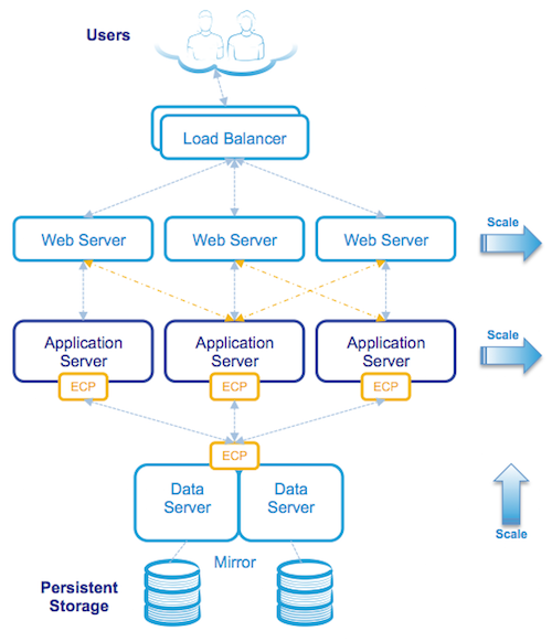
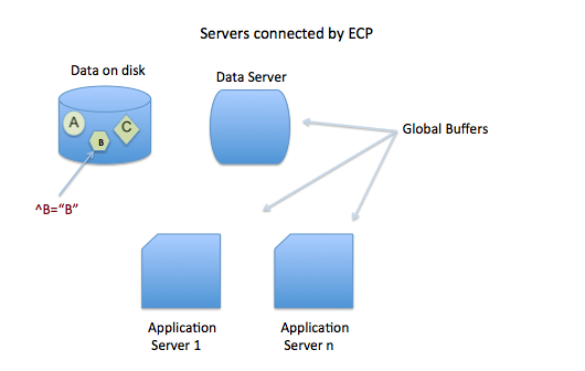
When I first started working with Caché, most customer operating systems were 32-bit, and memory for an IRIS application was limited and expensive. Commonly deployed Intel servers had only a few cores, and the only way to scale up was to go with big iron servers or use ECP to scale out horizontally. Now, even basic production-grade servers have multiple processors, dozens of cores, and minimum memory is hundreds of GB or TB. For most database installations, ECP is forgotten, and we can now scale application transaction rates massively on a single server.

A key feature of IRIS is the way we use data in shared memory usually referred to as database cache or global buffers. The short story is that if you can right size and allocate 'more' memory to global buffers you will usually improve system performance - data in memory is much faster to access than data on disk. Back in the day, when 32-bit systems ruled, the answer to the question how much memory should I allocate to global buffers? It was a simple - as much as possible! There wasn't that much available anyway, so sums were done diligently to calculate OS requirements, the number of and size of OS and IRIS processes and real memory used by each to find the remainder to allocate as large a global buffer as possible.

The tide has turned

If you are running your application on a current-generation server, you can allocate huge amounts of memory to an IRIS instance, and a laissez-faire attitude often applies because memory is now "cheap" and plentiful. However, the tide has turned again, and pretty much all but the very largest systems I see deployed now are virtualized. So, while 'monster' VMs can have large memory footprints if needed, the focus still comes back to the right sizing systems. To make the most of server consolidation, capacity planning is required to make the best use of available host memory.

What uses memory?

Generally, there are four main consumers of memory on an IRIS database server:

  • Operating System, including filesystem cache.
  • If installed, other non-IRIS applications.
  • IRIS processes.
  • IRIS shared memory (includes global and routine buffers and GMHEAP).

At a high level, the amount of physical memory required is simply added up by adding up the requirements of each of the items on the list. All of the above use real memory, but they can also use virtual memory. A key part of capacity planning is to size a system so that there is enough physical memory so that paging does not occur or is minimized, or at least minimize or eliminate hard page faults where memory has to be brought back from disk.

In this post I will focus on sizing IRIS shared memory and some general rules for optimising memory performance. The operating system and kernel requirements vary by operating system but will be several GB in most cases. File system cache varies and is will be whatever is available after the other items on the list take their allocation.

IRIS is mostly processes - if you look at the operating system statistics while your application is running you will see cache processes (e.g. iris or iris.exe). So a simple way to observe what your application memory requirements are is to look at the operating system metrics. For example with vmstat or ps on Linux or Windows process explorer and total the amount of real memory in use, extrapolating for growth and peak requirements. Be aware that some metrics report virtual memory which includes shared memory, so be careful to gather real memory requirements.

Sizing Global buffers - A simplified way

One of the capacity planning goals for a high transaction database is to size global buffers so that as much of the application database working set is in memory as possible. This will minimise read IOPS and generally improve the application's performance. We also need to strike a balance so that other memory users, such as the operating system and IRIS process, are not paged out and there is enough memory for the filesystem cache.

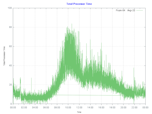
I showed an example of what can happen if reads from disk are excessive in Part 2 of this series. In that case, high reads were caused by a bad report or query, but the same effect can be seen if global buffers are too small, forcing the application to be constantly reading data blocks from disk. As a sidebar, it's also worth noting that the landscape for storage is always changing - storage is getting faster and faster with advances in SSDs and NVMe, but data in memory close to the running processes is still best.

Of course, every application is different, so it's important to say, "Your mileage may vary" but there are some general rules which will get you started on the road to capacity planning shared memory for your application. After that you can tune for your specific requirements.

Where to start?

Unfortunately, there is no magic answer. However, as I discussed in previous posts, a good practice is to size the system CPU capacity so that for a required peak transaction rate, the CPU will be approximately 80% utilized at peak processing times, leaving 20% headroom for short-term growth or unexpected spikes in activity.

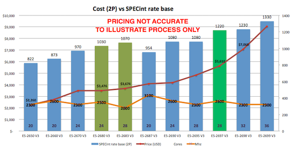
For example, when I am sizing TrakCare systems I know CPU requirements for a known transaction rate from benchmarking and reviewing customer site metrics, and I can use a broad rule of thumb for Intel processor-based servers:

Rule of thumb: Physical memory is sized at n GB per CPU core for servers running IRIS.

  • For example, for TrakCare database servers, a starting point of n is 8 GB. But this can vary, and servers may be right-sized after the application has been running for a while -- you must monitor your systems continuously and do a formal performance review, for example, every six or 12 months.

Rule of thumb: Allocate n% of memory to IRIS global buffers.

  • For small to medium TrakCare systems, n% is 60%, leaving 40% of memory for the operating system, filesystem cache, and IRIS processes. You may vary this, say to 50%, if you need a lot of filesystem cache or have a lot of processes. Or make it a higher percentage as you use very large memory configurations on large systems.
  • This rule of thumb assumes only one IRIS instance on the server.

For example, if the application needs 10 CPU cores, the VM would have 80 GB of memory, 48 GB for global buffers, and 32 GB for everything else.

Memory sizing rules apply to physical or virtualized systems, so the same 1 vCPU: 8 GB memory ratio applies to TrakCare VMs.

Tuning global buffers

There are a few items to observe to see how effective your sizing is. You can observe free memory outside IRIS with operating system tools. Set up as per your best calculations, then observe memory usage over time, and if there is always free memory, the system can be reconfigured to increase global buffers or to right-size a VM.

Another key indicator of good global buffer sizing is having read IOPS as low as possible, which means IRIS cache efficiency will be high. You can observe the impact of different global buffer sizes on PhyRds and RdRatio with mgstat; an example of looking at these metrics is in Part 2 of this series. Unless you have your entire database in memory, there will always be some reads from disk; the aim is simply to keep reads as low as possible.

Remember your hardware food groups and get the balance right. More memory for global buffers will lower read IOPS but possibly increase CPU utilization because your system can now do more work in a shorter time. Lowering IOPS is pretty much always a good thing, and your users will be happier with faster response times.

See the section below for applying your requirements to physical memory configuration.

For virtual servers, plan not to ever oversubscribe your production VM memory. This is especially true for IRIS shared memory; more on this below.

Is your application's sweet spot 8GB of physical memory per CPU core? I can't say, but see if a similar method works for your application, whether 4GB or 10GB per core. If you have found another method for sizing global buffers, please leave a comment below.

Monitoring Global Buffer usage

The IRIS utility ^GLOBUFF displays statistics about what your global buffers are doing at any point in time. For example to display the top 25 by percentage:

do display^GLOBUFF(25)

For example, output could look like this:

Total buffers: 2560000    Buffers in use: 2559981  PPG buffers: 1121 (0.044%)

Item  Global                             Database          Percentage (Count)
1     MyGlobal                           BUILD-MYDB1        29.283 (749651)
2     MyGlobal2                          BUILD-MYDB2        23.925 (612478)
3     CacheTemp.xxData                   CACHETEMP          19.974 (511335)
4     RTx                                BUILD-MYDB2        10.364 (265309)
5     TMP.CachedObjectD                  CACHETEMP          2.268 (58073)
6     TMP                                CACHETEMP          2.152 (55102)
7     RFRED                              BUILD-RB           2.087 (53428)
8     PANOTFRED                          BUILD-MYDB2        1.993 (51024)
9     PAPi                               BUILD-MYDB2        1.770 (45310)
10    HIT                                BUILD-MYDB2        1.396 (35727)
11    AHOMER                             BUILD-MYDB1        1.287 (32946)
12    IN                                 BUILD-DATA         0.803 (20550)
13    HIS                                BUILD-DATA         0.732 (18729)
14    FIRST                              BUILD-MYDB1        0.561 (14362)
15    GAMEi                              BUILD-DATA         0.264 (6748)
16    OF                                 BUILD-DATA         0.161 (4111)
17    HISLast                            BUILD-FROGS        0.102 (2616)
18    %Season                            CACHE              0.101 (2588)
19    WooHoo                             BUILD-DATA         0.101 (2573)
20    BLAHi                              BUILD-GECKOS       0.091 (2329)
21    CTPCP                              BUILD-DATA         0.059 (1505)
22    BLAHi                              BUILD-DATA         0.049 (1259)
23    Unknown                            CACHETEMP          0.048 (1222)
24    COD                                BUILD-DATA         0.047 (1192)
25    TMP.CachedObjectI                  CACHETEMP          0.032 (808)

This could be useful in several ways, for example, to see how much of your working set is kept in memory. If you find this utility is useful please make a comment below to enlighten other community users on why it helped you.

Sizing Routine Buffers

Routines your application is running, including compiled classes, are stored in routine buffers. The goal of sizing shared memory for routine buffers is for all your routine code to be loaded and stay resident in routine buffers. Like global buffers, it is expensive and inefficient to read routines off disk. The maximum size of routine buffers is 1023 MB. As a rule you want more routine buffers than you need as there is always a big performance gain to have routines cached.

Routine buffers are made up of different sizes. By default, IRIS determines the number of buffers for each size; at install time, the defaults for 2016.1 are 4, 16 and 64 KB. It is possible to change the allocation of memory for different sizes; however, to start your capacity planning, it is recommended to stay with IRIS defaults unless you have a special reason for changing. For more information, see routines in the IRIS documentation “config” appendix of the IRIS Parameter File Reference and Memory and Startup Settings in the “Configuring IRIS” chapter of the IRIS System Administration Guide.

As your application runs, routines are loaded off disk and stored in the smallest buffer the routine will fit. For example, if a routine is 3 KB, it will ideally be stored in a 4 KB buffer. If no 4 KB buffers are available, a larger one will be used. A routine larger than 32 KB will use as many 64 KB routine buffers as needed.

Checking Routine Buffer Use

mgstat metric RouLas

One way to understand if the routine buffer is large enough is the mgstat metric RouLas (routine loads and saves). A RouLas is a fetch from or save to disk. A high number of routine loads/saves may show up as a performance problem; in that case, you can improve performance by increasing the number of routine buffers.

cstat

If you have increased routine buffers to the maximum of 1023 MB and still find high RouLas a more detailed examination is available so you can see what routines are in buffers and how much is used with cstat command.

ccontrol stat cache -R1  

This will produce a listing of routine metrics including a list of routine buffers and all the routines in cache. For example a partial listing of a default IRIS install is:

Number of rtn buf: 4 KB-> 9600, 16 KB-> 7200, 64 KB-> 2400, 
gmaxrouvec (cache rtns/proc): 4 KB-> 276, 16 KB-> 276, 64 KB-> 276, 
gmaxinitalrouvec: 4 KB-> 276, 16 KB-> 276, 64 KB-> 276, 

Dumping Routine Buffer Pool Currently Inuse
 hash   buf  size sys sfn inuse old type   rcrc     rtime   rver rctentry rouname
   22: 8937  4096   0   1     1   0  D  6adcb49e  56e34d34    53 dcc5d477  %CSP.UI.Portal.ECP.0 
   36: 9374  4096   0   1     1   0  M  5c384cae  56e34d88    13 908224b5  %SYSTEM.WorkMgr.1 
   37: 9375  4096   0   1     1   0  D  a4d44485  56e34d88    22 91404e82  %SYSTEM.WorkMgr.0 
   44: 9455  4096   0   0     1   0  D  9976745d  56e34ca0    57 9699a880  SYS.Monitor.Health.x
 2691:16802 16384   0   0     7   0  P  da8d596f  56e34c80    27 383da785  START
   etc
   etc 	

"rtns/proc" on the 2nd line above is saying that 276 routines can be cached at each buffer size as default.

Using this information another approach to sizing routine buffers is to run your application and list the running routines with cstat -R1. You could then calculate the routine sizes in use, for example put this list in excel, sort by size and see exactly what routines are in use. If your are not using all buffers of each size then you have enough routine buffers, or if you are using all of each size then you need to increase routine buffers or can be more direct about configuring the number of each bucket size.

Lock table size

The locksiz configuration parameter is the size (in bytes) of memory allocated for managing locks for concurrency control to prevent different processes from changing a specific element of data at the same time. Internally, the in-memory lock table contains the current locks, along with information about the processes that hold those locks.

Since memory used to allocate locks is taken from GMHEAP, you cannot use more memory for locks than exists in GMHEAP. If you increase the size of locksiz, increase the size of GMHEAP to match as per the formula in the GMHEAP section below. Information about application use of the lock table can be monitored using the system management portal (SMP), or more directly with the API:

set x=##class(SYS.Lock).GetLockSpaceInfo().

This API returns three values: "Available Space, Usable Space, Used Space". Check Usable space and Used Space to roughly calculate suitable values (some lock space is reserved for lock structure). Further information is available in IRIS documentation.

Note: If you edit the locksiz setting, changes take place immediately.

GMHEAP

The GMHEAP (the Generic Memory Heap) configuration parameter is defined as: Size (in kilobytes) of the generic memory heap for IRIS. This is the allocation from which the Lock table, the NLS tables, and the PID table are also allocated.

Note: Changing GMHEAP requires a IRIS restart.

To assist you in sizing for your application information about GMHEAP usage can be checked using the API:

%SYSTEM.Config.SharedMemoryHeap

This API also provides the ability to get available generic memory heap and recommends GMHEAP parameters for configuration. For example, the DisplayUsage method displays all memory used by each of the system components and the amount of available heap memory. Further information is available in the IRIS documentation.

write $system.Config.SharedMemoryHeap.DisplayUsage()

The RecommendedSize method can give you an idea of GMHEAP usage and recommendations at any point in time. However, you will need to run this multiple times to build up a baseline and recommendations for your system.

write $system.Config.SharedMemoryHeap.RecommendedSize()

Rule of thumb: Once again your application mileage will vary, but somewhere to start your sizing could be one of the following:

(Minimum 128MB) or (64 MB * number of cores) or (2x locksiz) or whichever is larger.

Remember GMHEAP must be sized to include the lock table. 

Large/Huge pages

The short story is that huge pages on Linux have a positive effect on increasing system performance. However, the benefits will only be known if you test your application with and without huge pages. The benefits of huge pages for IRIS database servers are more than just performance -- which may only be ~10% improvement at best. There are other reasons to use huge pages; When IRIS uses huge pages for shared memory, you guarantee that the memory is available for shared memory and not fragmented.

Note: By default, when huge/large pages are configured, InterSystems IRIS attempts to utilize them on startup. If there is not enough space, InterSystems IRIS reverts to standard pages. However, you can use the memlock parameter to control this behavior and fail at startup if huge/large page allocation fails.

As a sidebar for TrakCare, we do not automatically specify huge pages for non-production servers/VMs with small memory footprints ( for example less than 8GB) or utility servers (for example print servers) running IRIS because allocating memory for huge pages may end up orphaning memory, or sometimes a bad calculation that undersizes huge pages means IRIS starts not using huge pages which is even worse. As per our docs, remember that when using huge pages to configure and start IRIS without huge pages, look at the total shared memory at startup and then use that to calculate huge pages. Configuring Huge and Large Pages

Danger! Windows Large Pages and Shared Memory

IRIS uses shared memory on all platforms and versions, and it's a great performance booster, including on Windows, where it is always used. However, there are particular issues unique to Windows that you need to be aware of.

When IRIS starts, it allocates a single, large chunk of shared memory to be used for database cache (global buffers), routine cache (routine buffers), the shared memory heap, journal buffers, and other control structures. On IRIS startup, shared memory can be allocated using small or large pages. On Windows 2008 R2 and later, IRIS uses large pages by default; however, if a system has been running for a long time, due to fragmentation, contiguous memory may not be able to be allocated at IRIS startup, and IRIS can instead start using small pages.

Unexpectedly starting IRIS with small pages can cause it to start with less shared memory than defined in the configuration, or it may take a long time to start or fail to start. I have seen this happen on sites with a failover cluster where the backup server has not been used as a database server for a long time.

Tip: One mitigation strategy is periodically rebooting the offline Windows cluster server. Another is to use Linux.

Physical Memory

The best configuration for the processor dictates physical memory. A bad memory configuration can significantly impact performance.

Intel Memory configuration best practice

This information applies to Intel processors only. Please confirm with vendors what rules apply to other processors.

Factors that determine optimal DIMM performance include:

  • DIMM type
  • DIMM rank
  • Clock speed
  • Position to the processor (closest/furthest)
  • Number of memory channels
  • Desired redundancy features.

For example, on Nehalem and Westmere servers (Xeon 5500 and 5600) there are three memory channels per processor and memory should be installed in sets of three per processor. For current processors (for example, E5-2600), there are four memory channels per processor, so memory should be installed in sets of four per processor.

When there are unbalanced memory configurations — where memory is not installed in sets of three/four or memory DIMMS are different sizes, unbalanced memory can impose a 23% memory performance penalty.

Remember that one of the features of IRIS is in-memory data processing, so getting the best performance from memory is important. It is also worth noting that for maximum bandwidth servers should be configured for the fastest memory speed. For Xeon processors maximum memory performance is only supported at up to 2 DIMMs per channel, so the maximum memory configurations for common servers with 2 CPUs is dictated by factors including CPU frequency and DIMM size (8GB, 16GB, etc).

Rules of thumb:

  • Use a balanced platform configuration: populate the same number of DIMMs for each channel and each socket
  • Use identical DIMM types throughout the platform: same size, speed, and number of ranks.
  • For physical servers, round up the total physical memory in a host server to the natural break points—64GB, 128GB, and so on—based on these Intel processor best practices.

VMware Virtualisation considerations

I will follow up in future with another post with more guidelines for when IRIS is virtualized. However the following key rule should be considered for memory allocation:

Rule: Set VMware memory reservation on production systems.

As we have seen above when IRIS starts, it allocates a single, large chunk of shared memory to be used for global and routine buffers, GMHEAP, journal buffers, and other control structures.

You want to avoid any swapping for shared memory so set your production database VMs memory reservation to at least the size of IRIS shared memory plus memory for IRIS processes and operating system and kernel services. If in doubt reserve the full production database VMs memory.

As a rule if you mix production and non-production servers on the same systems do not set memory reservations on non-production systems. Let non-production servers fight out whatever memory is left ;). VMware often calls VMs with more than 8 CPUs 'monster VMs'. High transaction IRIS database servers are often monster VMs. There are other considerations for setting memory reservations on monster VMs, for example if a monster VM is to be migrated for maintenance or due to a High Availability triggered restart then the target host server must have sufficient free memory. There are stratagies to plan for this I will talk about them in a future post along with other memory considerations such as planning to make best use of NUMA.

Summary

This is a start to capacity planning memory, a messy area - certainly not as clear cut as sizing CPU. If you have any questions or observations please leave a comment.

As this entry is posted I am on my way to Global Summit 2016. If you are attending this year I will be talking about performance topics with two presentations, or I am happy to catch up with you in person in the developers area.

3
9 11083
Article Murray Oldfield · Nov 25, 2016 23m read

Hyper-Converged Infrastructure (HCI) solutions have been gaining traction for the last few years with the number of deployments now increasing rapidly. IT decision makers are considering HCI when scoping new deployments or hardware refreshes especially for applications already virtualised on VMware. Reasons for choosing HCI include; dealing with a single vendor, validated interoperability between all hardware and software components, high performance especially IO, simple scalability by addition of hosts, simplified deployment and simplified management.

I have written this post with an introduction for a reader who is new to HCI by looking at common features of HCI solutions. I then review configuration choices and recommendations for capacity planning and performance when deploying applications built on InterSystems data platform with specific examples for database applications. HCI solutions rely on flash storage for performance so I also include a section on characteristics and use cases of selected flash storage options.

Capacity planning and performance recommendations in this post are specific to VMWare vSAN. However vSAN is not alone in the growing HCI market, there are other HCI vendors, notably Nutanix which also has an increasing number of deployments. There is a lot of commonality between features no matter which HCI vendor you choose so I expect the recommendations in this post are broadly relevant. But the best advice in all cases is to discuss the recommendations from this post with HCI vendors taking into account your application specific requirements.


[A list of other posts in the InterSystems Data Platforms and performance series is here.](https://community.intersystems.com/post/capacity-planning-and-performance-series-index)
# What is HCI?

Strictly speaking converged solutions have been around for a long time, however in this post I am talking about current HCI solutions for example from Wikipedia: "Hyperconvergence moves away from multiple discrete systems that are packaged together and evolve into software-defined intelligent environments that all run in commodity, off-the-shelf x86 rack servers...."

So is HCI a single thing?

No. When talking to vendors you must remember HCI has many permutations; Converged and Hyper-converged are more a type of architecture not a specific blueprint or standard. Due to the commodity nature of HCI hardware the market has multiple vendors differentiating themselves at the software layer and/or other innovative ways of combining compute, network, storage and management.

Without going down too much of a rat hole here, as an example solutions labeled HCI can have storage inside the servers in a cluster or have more traditional configuration with a cluster of servers and separate SAN storage -- possibly from different vendors -- that has also been tested and validated for interoperability and managed from a single control plane. For capacity and performance planning you must consider solutions where storage is in an array connected over a SAN fabric (e.g. Fibre Channel or Ethernet) have a different performance profile and requirements to the case where the storage pool is software defined and located inside each of a cluster of server nodes with storage processing on the servers.

So what is HCI again?

For this post I am focusing on HCI and specifically VMware vSAN where storage is physically inside the host servers. In these solutions the HCI software layer enables the internal storage in each of multiple nodes in a cluster performing processing to act like one shared storage system. So another driver of HCI is even though there is a cost for HCI software there could also be significant savings using HCI when compared to solutions using enterprise storage arrays.

For this post I am talking about solutions where HCI combines compute, memory, storage, network and management software into a cluster of virtualised x86 servers.

Common HCI characteristics

As mentioned above VMWare vSAN and Nutanix are examples of HCI solutions. Both have similar high level approaches to HCI and are good examples of the format:

  • VMware vSAN requires VMware vSphere and is available on multiple vendors hardware. There are many hardware choices available but these are strictly dependent on VMware's vSAN Hardware Compatibility List (HCL). Solutions can be purchased prepackaged and preconfigured for example EMC VxRail or you can purchase components on the HCL and build-your-own.
  • Nutanix can also be purchased and deployed as an all-in-one solution including hardware in preconfigured blocks with up to four nodes in a 2U appliance. Nutanix solution is also available as a build-your-own software solution validated on other vendors hardware.

There are some variations in implementation, but generally speaking HCI have common features that will inform your planning for performance and capacity:

  • Virtual Machines (VMs) run on hypervisors such as VMware ESXi but also others including Hyper-V or Nutanix Acropolis Hypervisor (AHV). Nutanix can also be deployed using ESXi.
  • Host servers are often combined into blocks of compute, storage and network. For example a 2U Appliance with four nodes.
  • Multiple host servers are combined into a cluster for management and availability.
  • Storage is tiered, either all-flash or a hybrid with a flash cache tier plus spinning disks as a capacity tier.
  • Storage is presented as a pool which is software defined including data placement and policies for capacity, performance and availability.
  • Capacity and IO performance are scaled by adding hosts to the cluster.
  • Data is written to storage on multiple cluster nodes synchronously so the cluster can tolerate host or component failures without data loss.
  • VM availability and load balancing is provided by the hypervisor for example vMotion, VMware HA, and DRS.

As I noted above there are also other HCI solutions with twists on this list such as support for external storage arrays, storage only nodes... the list is a long as the list of vendors.

HCI adoption is gathering pace and competition between the vendors is driving innovation and performance improvements. It is also worth noting that HCI is a basic building block for cloud deployment.


# Are InterSystems' products supported on HCI?

It is InterSystems policy and procedure to verify and release InterSystems’ products against processor types and operating systems including when operating systems are virtualised. Please note InterSystems Advisory: Software Defined Data Centers (SDDC) and Hyper-Converged Infrastructure (HCI).

For example: Caché 2016.1 running on Red Hat 7.2 operating system on vSAN on x86 hosts is supported.

Note: If you do not write your own applications you must also check your application vendors support policy.


# vSAN Capacity Planning

This section highlights considerations and recommendations for deployment of VMware vSAN for database applications on InterSystems data platforms -- Caché, Ensemble and HealthShare. However you can also use these recommendations as a general list of configuration questions for reviewing with any HCI vendor.


VM vCPU and memory

As a starting point use the same capacity planning rules for your database VMs' vCPU and memory as you already use for deploying your applications on VMware ESXi with the same processors.

As a refresher for general CPU and memory sizing for Caché a list of other posts in this series is here: Capacity planning and performance series index.

One of the features of HCI systems is very low storage IO latency and high IOPS capability. You may remember from the 2nd post in this series the hardware food groups graphic showing CPU, memory, storage and network. I pointed out that these components are all related to each other and changes to one component can affect another, sometimes with unexpected consequences. For example I have seen a case of fixing a particularly bad IO bottleneck in a storage array caused CPU usage to jump to 100% resulting in even worse user experience as the system was suddenly free to do more work but did not have the CPU resources to service increased user activity and throughput. This effect is something to bear in mind when you are planning your new systems if your sizing model is based on performance metrics from less performant hardware. Even though you will be upgrading to newer servers with newer processors your database VM activity must be monitored closely in case you need to right-size due to lower latency IO on the new platform.

Also note, as detailed later you will also have to account for software defined storage IO processing when sizing physical host CPU and memory resources.


Storage capacity planning

To understand storage capacity planning and put database recommendations in context you must first understand some basic differences between vSAN and traditional ESXi storage. I will cover these first then break down all the best practice recommendations for Caché databases.

vSAN storage model

At the heart of vSAN and HCI in general is software defined storage (SDS). The way data is stored and managed is very different to using a cluster of ESXi servers and a shared storage array. One of the advantages of HCI is there are no LUNs, instead pool(s) of storage that are allocated to VMs as needed with policies describing capabilities for availability, capacity, and performance per-VMDK.

For example; imagine a traditional storage array consisting of shelves of physical disks configured together as various sized disk groups or disk pools with different numbers and/or types of disk depending on performance and availability requirements. Disk groups are then presented as a number of logical disks (storage array volumes or LUNs) which are in turn presented to ESXi hosts as datastores and are formatted as VMFS volumes. VMs are represented as files in the datastores. Database best practice for availability and performance recommends at minimum separate disk groups and LUNs for database (random access), journals (sequential), and any others (such as backups or non-production systems, etc).

vSAN is different; storage from the vSAN is allocated using storage policy-based management (SPBM). Policies can be created using combinations of capabilities, including the following (but there are more);

  • Failures To Tolerate (FTT) which dictates the number of redundant copies of data.
  • Erasure coding (RAID-5 or RAID-6) for space savings.
  • Disk stripes for performance.
  • Thick or thin disk provisioning (thin by default on vSAN).
  • Others...

VMDKs (individual VM disks) are created from the vSAN storage pool by selecting appropriate policies. So instead of creating disk groups and LUNs on the array with a set attributes, you define the capabilities of storage as policies in vSAN using SPBM; for example "Database" would be different to "Journal", or whatever others you need. You set the capacity and select the appropriate policy when you create disks for your VM.

Another key concept is a VM is no longer a set of files on a VMDK datastore but is stored as a set of storage objects. For example your database VM will be made up of multiple objects and components including the VMDKs, swap, snapshots, etc. vSAN SDS manages all the mechanics of object placement to meet the requirements of the policies you selected.


Storage tiers and IO performance planning

To ensure high performance there are two tiers of storage;

  • Cache tier - Must be high endurance flash.
  • Capacity tier - Flash or for hybrid uses spinning disks.

As shown in the graphic below storage is divided into tiers and disk groups. In vSAN 6.5 each disk group includes a single cache device and up to seven spinning disks or flash devices. There can be up to five disk groups so possibly up to 35 devices per host. The figure below shows an all-flash vSAN cluster with four hosts, each host has two disk groups each with one NVMe cache disk and three SATA capacity disks.


vSAN all-flash storage example

Figure 1. vSAN all-flash storage showing tiers and disk groups


When considering how to populate tiers and the type of flash for cache and capacity tiers you must consider the IO path; for the lowest latency and maximum performance writes go to the cache tier then software coalesces and de-stages the writes to the capacity tier. Cache use depends on deployment model, for example in vSAN hybrid configurations 30% of the cache tier is write cache, in the case of all-flash 100% of cache tier is write cache -- reads are from low latency flash capacity tier.

There will be a performance boost using all-flash. With larger capacity and durable flash drives available today the time has come where you should be considering whether you need spinning disks. The business case for flash over spinning disk has been made over recent years and includes much lower cost/IOPS, performance (lower latency), higher reliability (no moving parts to fail, less disks to fail for required IOPS), lower power and heat profile, smaller footprint, and so on. You will also benefit from additional HCI features, for example vSAN will only allow deduplication and compression on all-flash configurations.

  • Recommendation: For best performance and lower TCO consider all-flash.

For best performance the cache tier should have the lowest latency, especially for vSAN as there is only a single cache device per disk group.

  • Recommendation: If possible choose NVMe SSDs for the cache tier although SAS is still OK.
  • Recommendation: Choose high endurance flash devices in the cache tier to handle high I/O.

For SSDs at the capacity tier there is negligible performance difference between SAS and SATA SSDs. You do not need to incur the cost of NVMe SSD at the capacity tier for database applications. However in all cases ensure you are using enterprise class SATA SSDs with features such as power failure protection.

  • Recommendation: Choose high capacity SATA SSDs for capacity tier.
  • Recommendation: Choose enterprise SSDs with power failure protection.

Depending on your timetable new technologies such as such as 3D Xpoint with higher IOPS, lower latency, higher capacity and higher durability may be available. There is a breakdown of flash storage at the end of this post.

  • Recommendation: Watch for new technologies to include such as 3D Xpoint for cache AND capacity tier.

As I mentioned above you can have up to five disk groups per host and a disk group is made up of one flash device and up to seven devices at the capacity tier. You could have a single disk group with one flash device and as much capacity as you need, or multiple disk groups per host. There are advantages to having multiple disk groups per host:

  • Performance: Having multiple flash devices at the tiers will increase the IOPS available per host.
  • Failure domain: Failure of a cache disk impacts the entire disk group, although availability is maintained as vSAN rebuilds automatically.

You will have to balance availability, performance and capacity, but in general having multiple disk groups per host is a good balance.

  • Recommendation: Review storage requirements, consider multiple disk groups per host.

What performance should I expect?

A key requirement for good application user experience is low storage latency; the usual recommendation is that database read IO latency should be below 10ms. Refer to the table from Part 6 of this series here for details.

For Caché database workloads tested using the default vSAN storage policy and Caché RANREAD utility I have observed sustained 100% random read IO over 30K IOPS with less than 1ms latency for all-flash vSAN using Intel S3610 SATA SSDs at the capacity tier. Considering that a basic rule of thumb for Caché databases is to size instances to use memory for as much database IO as possible all-flash latency and IOPS capability should provide ample headroom for most applications. Remember memory access times are still orders of magnitude lower than even NVMe flash storage.

As always remember your mileage will vary; storage policies, number of disk groups and number and type of disks etc will influence performance so you must validate on your own systems!


Capacity and performance planning

You can calculate the raw TB capacity of a vSAN storage pool roughly as the total size of disks in the capacity tier. In our example configuration in figure 1 there are a total of 24 x INTEL S3610 1.6TB SSDs:

Raw capacity of cluster: 24 x 1.6TB = 38.4 TB

However available capacity is much different and where calculations get messy and is dependent on configuration choices; which policies are used (such as FTT which dictates how many copies of data) and also whether deduplication and compression have been enabled.

I will step through selected policies and discuss their implications for capacity and performance and recommendations for a database workload.

All ESXi deployments I see are made up of multiple VMs; for example, TrakCare a unified healthcare information system built on InterSystems’ health informatics platform, HealthShare is at its heart at least one large (monster) database server VM which is absolutely fits the description "tier-1 business critical application". However a deployment also includes combinations of other single purpose VMs such as production web servers, print servers, etc. As well as test, training and other non-production VMs. Usually all deployed in a single ESXi cluster. While I focus on database VM requirements remember that SPBM can be tailored per VMDK for all your VMs.

Deduplication and Compression

For vSAN deduplication and compression is a cluster-wide on/off setting. Deduplication and compression can only be enabled when you are using an all-flash configuration. Both features are enabled together.

At first glance deduplication and compression seems to be a good idea - you want to save space, especially if you are using (more expensive) flash devices at the capacity tier. While there are space savings with deduplication and compression my recommendation is that you do not enable this feature for clusters with large production databases or where data is constantly being overwritten.

Deduplication and compression does add some processing overhead on the host, maybe in the range of single digit %CPU utilization, but this is not the primary reason not recommending for databases.

In summary vSAN attempts to deduplicate data as it is written to the capacity tier within the scope of a single disk group using 4K blocks. So in our example at figure 1 data objects to be deduplicated would have to exists in the capacity tier of the same disk group. I am not convinced we will see much savings on Caché database files which are basically very large files filled with 8K database blocks with unique pointers, contents, etc. Secondly vSAN will only attempt to compress duplicated blocks, and will only consider blocks compressed if compression reaches 50% or more. If the deduplicated block does not compress to 2K it is written uncompressed. While there may be some duplication of operating system or other files the real benefit of deduplication and compression would be for clusters deployed for VDI.

Another caveat is the impact of a (albeit rare) failure of one device in a disk group on the whole group when deduplication and compression is on. The whole disk group is marked "unhealthy" which has a cluster wide impact: because the group is marked unhealthy all the data on a disk group will be evacuated off that group to other places, then the device must be replaced and vSAN will resynchronise the objects to rebalance.

  • Recommendation: For database deployments do not enable compression and deduplication.

Sidebar: InterSystems database mirroring.

For mission critical tier-1 Caché database application instances requiring the highest availability I recommend InterSystems synchronous database mirroring, even when virtualised. Virtualised solutions have HA built in; for example VMWare HA, however additional advantages of also using mirroring include:

  • Separate copies of up-to-date data.
  • Failover in seconds (faster than restarting a VM then operating System then recovering Caché).
  • Failover in case of application/Caché failure (not detected by VMware).

I am guessing you have spotted the flaw in enabling deduplication when you have mirrored databases on the same cluster? You will be attempting to deduplicate your mirror data. Generally not sensible and also a processing overhead.

Another consideration when deciding whether to mirror databases on HCI is the total storage capacity required. vSAN will be making multiple copies of data for availability, this data storage will be doubled again by mirroring. You will need to weigh the small incremental increase in uptime over what VMware HA provides against the additional cost of storage.

For maximum uptime you can create two clusters so that each node of the database mirror is in a completely independent failure domain. However take note of the total servers and storage capacity to provide this level of uptime.


Encryption

Another consideration is where you choose to encrypt data at rest. You have several choices in the IO stack including;

  • Using Caché database encryption (encrypts database only).
  • At Storage (e.g. hardware disk encryption at SSD).

Encryption will have a very small impact on performance, but can have a big impact on capacity if you choose to enable deduplication or compression in HCI. If you do choose deduplication and/or compression you would not want to be using Caché database encryption because it would negate any gains as encrypted data is random by design and does not compress well. Consider the protection point or risk they are trying to protect from, for example theft of file vs. theft of device.

  • Recommendation: Encrypt at the lowest layer as possible in the IO stack for a minimal level of encryption. However the more risk you want to protect move higher up the stack.

Failures To Tolerate (FTT)

FTT sets a requirement on the storage object to tolerate at least n number of concurrent host, network, or disk failures in the cluster and still ensure the availability of the object. The default is 1 (RAID-1); the VM’s storage objects (e.g. VMDK) are mirrored across ESXi hosts.

So vSAN configuration must contain at least n + 1 replicas (copies of the data) which also means there are 2n + 1 hosts in the cluster.

For example to comply with a number of failures to tolerate = 1 policy, you need three hosts at a minimum at all times -- even if one host fails. So to account for maintenance or other times when a host is taken off-line you need four hosts.

  • Recommendation: A vSAN cluster must have a minimum four hosts for availability.

Note there is also exceptions; a Remote Office Branch Office (ROBO) configuration that is designed for two hosts and a remote witness VM.


Erasure Coding

The default storage method on vSAN is RAID-1 -- data replication or mirroring. Erasure coding is RAID-5 or RAID-6 with storage objects/components distributed across storage nodes in the cluster. The main benefit of erasure coding is better space efficiency for the same level of data protection.

Using the calculation for FTT in the previous section as an example; for a VM to tolerate two failures using a RAID-1 there must be three copies of storage objects meaning a VMDK will consume 300% of the base VMDK size. RAID-6 also allows a VM to tolerate two failures and only consumes 150% the size of the VMDK.

The choice here is between performance and capacity. While the space saving is welcome you should consider your database IO patterns before enabling erasure coding. Space efficiency benefits come at the price of the amplification of I/O operations which is higher again during times of component failure so for best database performance use RAID-1.

  • Recommendation: For production databases do not enable erasure coding. Enable for non-production.

Erasure coding also impacts the number of hosts required in your cluster. For for example for RAID-5 you need a minimum of four nodes in the cluster, for RAID-6, you need a minimum of six nodes.

  • Recommendation: Consider the cost of additional hosts before planning to configure erasure coding.

Striping

Striping offers opportunity for performance improvements but will likely only help with hybrid configurations.

  • Recommendation: For production databases do not enable striping.

Object Space Reservation (thin or thick provisioning)

The name for this setting comes from vSAN using objects to store components of your VMs (VMDKs etc). By default all VMs provisioned to a VSAN datastore have object space reservation of 0% (thin provisioned) which leads to space savings and also enables vSAN more freedom for placement of data. However for your production databases best practice is to use 100% reservation(thick provisioned) where space is allocated at creation. For vSAN this will be Lazy Zeroed – where 0’s are written as each block is first written to. There are a few reasons for choosing 100% reservation for production databases; there will be less delay when database expansions occur, and you are guaranteeing that storage will be available when you need it.

  • Recommendation: For production database disks use 100% reservation.
  • Recommendation: For non-production instances leave storage thin provisioned.

When should I turn on features?

You can generally enable availability and space saving features after using the systems for some time, that is; when there are active VMs and users on the system. However there will be performance and capacity impact. Additional replicas of data in addition to the original are needed so additional space is required while data is synchronised. My experience is that enabling these type of features on clusters with large databases can take a very long time and expose the possibility of reduced availability.

  • Recommendation: Spend time up front to understand and configure storage features and functionality such as deduplication and compression before go-live and definitely before large databases are loaded.

There are other considerations such as leaving free space for disk balancing, failure etc. The point is you will have to take into account the recommendations in this post with vendor specific choices to understand your raw disk requirements.

  • Recommendation: There are many features and permutations. Work out your total GB capacity requirements as a starting point, review recommendations in this post [and with your application vendor] then talk to your HCI vendor.

Storage processing overhead

You must consider the overhead of storage processing on the hosts. Storage processing otherwise handled by the processors on an enterprise storage array is now being computed on each host in the cluster.

The amount of overhead per host will be dependent on workload and what storage features are enabled. My observations with basic testing I have done with Caché on vSAN shows that processing requirements are not excessive, especially when you consider the number of cores available on current servers. VMware recommends planning for 5-10% host CPU usage

The above can be a starting point for sizing but remember your mileage will vary and you will need to confirm.

  • Recommendation: Plan for worst case of 10% CPU utilisation and then monitor your real workload.

Network

Review vendor requirements -- assume minimum 10GbE NICs -- multiple NICs for storage traffic, management (e.g. vMotion), etc. I can tell you from painful experience that an enterprise class network switch is required for optimal operation of the cluster -- after all - all writes are sent synchronously over the network for availability.

  • Recommendation: Minimum 10GbE switched network bandwidth for storage traffic. Multiple NICs per host as per best practice.

Flash Storage Overview

Flash storage is a requirement of HCI so it is good to review where flash storage is today and where its going in the near future.

The short story is whether you use HCI or not if you are not deploying your applications using storage with flash today it is likely that your next storage purchase will include flash.

Storage today and tomorrow

Let us review the capabilities of commonly deployed storage solutions and be sure we are clear with the terminology.

Spinning disk

  • Old faithful. 7.2, 10K or 15K HDD spinning disks with SAS or SATA interface. Low IOPS per disk. Can be high capacity but that means the IOPS per GB are decreasing. For performance typically data is striped across multiple disks to achieve 'just enough' IOPS with high capacity.

SSD disk - SATA and SAS

  • Today flash is usually deployed as SAS or SATA interface SSDs using NAND flash. There is also some DRAM in the SSD as a write buffer. Enterprise SSDs include power loss protection - in event of power failure contents of DRAM are flushed to NAND.

SSD disk - NVMe

  • Similar to SSD disk but uses NVMe protocol (not SAS or SATA) with NAND flash. NVMe media attach via PCI Express (PCIe) bus allowing the system to talk directly without the overhead of host bus adapters and storage fabrics resulting in much lower latency.

Storage Array

  • Enterprise Arrays provide protection and the ability to scale. It is more common today that storage is either a hybrid array or all-flash. Hybrid arrays have a cache tier of NAND flash plus one or more capacity tiers using 7.2, 10K or 15K spinning disks. NVMe arrays are also becoming available.

Block-Mode NVDIMM

  • These devices are shipping today and are used when extremely low latencies are required. NVDIMMs sit in a DDR memory socket and provide latencies around 30ns. Today they ship in 8GB modules so are not likely to be used for legacy database applications, but new scale-out applications may take advantage of this performance.

3D XPoint

This is a future technology - not available in November 2016.

  • Developed by Micron and Intel. Also known as Optane (Intel) and QuantX (Micron).
  • Will not be available until at least 2017 but compared to NAND promises higher capacity, >10x more IOPS, >10x lower latency with extremely high Endurance and consistent performance.
  • First availability will use NVMe protocol.

SSD device Endurance

SSD device endurance is an important consideration when choosing drives for cache and capacity tiers. The short story is that flash storage has a finite life. Flash cells in an SSD can only be deleted and rewritten a certain number of times (no restrictions apply to reads). Firmware in the device manages spreading writes around the drive to maximise the life of the SSD. Enterprise SSDs also typically have more real flash capacity than visible to achieve longer life (over-provisioned), for example an 800GB drive may have more than 1TB of flash.

The metric to look for and discuss with your storage vendor is full Drive Writes Per Day (DWPD) guaranteed for a certain number of years. For example; An 800GB SSD at 1 DWPD for 5 years can have 800GB per day written for 5 years. So the higher the DWPD (and years) the higher the endurance. Another metric simply switches the calculation to show SSD devices specified in Terabytes Written (TBW); The same example has TBW of 1,460 TB (800GB * 365 days * 5 years). Either way you get an idea of the life of the SSD based on your expected IO.


Summary

This post covers the most important features to consider when deploying HCI and specifically VMWare vSAN version 6.5. There are vSAN features I have not not covered, if I have not mentioned a feature assume you should use the defaults. However if you have any questions or observations I am happy to discuss via the comments section.

I expect to return to HCI in future posts, this certainly is an architecture that is on the upswing so I expect to see more InterSystems customers deploying on HCI.


7
1 3753
Article Murray Oldfield · Oct 1, 2016 10m read

One of the great availability and scaling features of Caché is Enterprise Cache Protocol (ECP). With consideration during application development distributed processing using ECP allows a scale out architecture for Caché applications. Application processing can scale to very high rates from a single application server to the processing power of up to 255 application servers with no application changes.

ECP was used widely for many years in TrakCare deployments I was involved in. A decade ago a 'big' x86 server from one of the major vendors might only have a total of eight cores. For larger deployments ECP was a way to scale out processing on commodity servers rather than a single large and expensive big iron enterprise server. Even the high core count enterprise servers had limits so ECP was also used to scale deployments on them as well.

Today most new TrakCare deployments or upgrades to current hardware do not require ECP for scaling. Current two-socket x86 production servers can have dozens of cores and huge memory. We see that with recent Caché versions TrakCare -- and many other Caché applications -- have predictable linear scaling with the ability to support incremental increases in users and transactions as CPU core counts and memory increase in a single server. In the field I see most new deployments are virtualised, even then VMs can scale as needed up to the size of the host server. If resource requirements are more than a single physical host can provide then ECP is used to scale out.

  • Tip:For simplified management and deployment scale within a single server before deploying ECP.

In this post I will show an example architecture and the basics of how ECP works then review performance considerations with a focus on storage.

Specific information on configuring ECP and application development is available in the online Caché Distributed Data Management Guide and there is an ECP learning track here on the community.

One of the other key features of ECP is increasing application availability, for details see the ECP section in the Caché high availability guide.


[A list of other posts in this series is here](https://community.intersystems.com/post/capacity-planning-and-performance-series-index)
# ECP Architecture Basics

The architecture and operation of ECP is conceptually simple, ECP provides a way to efficiently share data, locks, and executable code among multiple server systems. Viewed from the application server data and code are stored remotely on a Data server, but are cached in memory locally on the Application servers to provide efficient access to active data with minimal network traffic.

The Data server manages database reads and writes to persistent storage on disk while multiple Application servers are the workhorses of the solution performing most of the application processing.

Multi-tier architecture

ECP is a multi-tier architecture. There are different ways to describe processing tiers and the roles they perform, the following is what I find useful when describing web browser based Caché applications and is the model and terminology for my posts. I appreciate that there may be different ways to break down tiers, but for now lets use my way :)

A browser based application, for example using Caché Server Pages (CSP) uses a multi-tier architecture where presentation, application processing, and data management functions are logically separated. Logical 'servers' with different roles populate the tiers. Logical servers do not have to be kept on separate physical host or virtual servers, for cost effectiveness and manageability some or even all logical servers may be located on a single host or operating system instance. As deployments scale up servers may be split out to multiple physical or virtual hosts with ECP so spreading the processing workload as needed without change to the application.

Host systems may be physical or virtualised depending on your capacity and availability requirements. The following tiers and logical servers make up a deployment:

  • Presentation Tier: Includes the Web Server which acts as gateway between the browser-based clients and the application tier.
  • Application Tier: This is where the ECP Application server sits. As noted above this is a logical model where the application server does not have to be separate from the Data server, and are typically not required to be for all but the largest sites. This tier may also include other servers for specialised processing such as report servers.
  • Data Tier: This is where the Data server is located. The data server performs transaction processing and is the repository for application code and data stored in the Caché database. The Data Server is responsible for reading and writing to persistent disk storage.

Logical Architecture

The following diagram is a logical view of a browser based application when deployed as a three-tier architecture:

Although at first glance the architecture may look complicated it is still made up of the same components as a Caché system installed on a single server, but with the logical components installed on multiple physical or virtual servers. All communication between servers is via TCP/IP.

ECP Operation in the logical view

Starting from the top the diagram above shows users connecting securely to multiple load balanced web servers. The web servers pass CSP web page requests between the clients and the application tier (the Application servers) which perform any processing, allowing content to be created dynamically, and returns the completed page back to the client via the web server.

In this three-tier model application processing has been spread over multiple Application servers using ECP. The application simply treats the data (your application database) as if it was local to the Application server.

When an Application server makes a request for data it will attempt to satisfy the request from its local cache, if it cannot, ECP will request the necessary data from the Data server which may be able to satisfy the request from its own cache or if not will fetch the data from disk. The reply from the Data server to the Application server includes the database block(s) where that data was stored. These blocks are used and now cached on the Application server. ECP automatically takes care of managing cache consistency across the network and propagating changes back to the Data server. Clients enjoy fast responses because they frequently use locally cached data.

By default web servers communicate with a preferred Application server ensuring that the same Application server services subsequent requests for related data as the data is likely to already be in local cache.

  • Tip:As detailed in the Caché documentation avoid connecting users to application servers in a round-robin or load-balancing scheme wich impacts the benefit of caching on the application server. Ideally the same users or groups of users stay connected to the same application server.

The solution is scaled without user downtime at the Presentation Tier by adding web servers and at the Application Tier by adding additional Application servers. The Data tier is scaled by increasing CPU and memory on the Data servers.

Physical Architecture

The following diagram shows an example of physical hosts used in the same three-tier deployment as the three-tier logical architecture example:

Note that physical or virtualised hosts are deployed at each tier using an n+1 or n+2 model for 100% capacity in event of a host failure or scheduled maintenance. Because users are spread across multiple web and application servers, the failure of a single server affects a smaller population with users automatically reconnecting to one of the remaining servers.

The Data management tier is made highly available, for example located on a failover cluster (e.g. virtualization HA, InterSystems Database Mirroring, or traditional failover clustering) connected to one or more storage arrays. In the event of hardware or service failure clustering will restart the services on one of the surviving nodes in the cluster. As an added benefit, ECP has built-in resiliency and maintains transactional integrity in the event of a database node cluster failover, application users will observe a pause in processing until failover and automatic recovery completes and users then seamlessly resume without disconnection.

The same architecture can also be mapped to virtualised servers, for example VMware vSphere can be used to virtualise Application servers.

ECP Capacity Planning

As noted above the Data server manages database reads and writes to persistent disk while multiple Application servers are the workhorses of the solution performing most of the application processing. This is a key concept when considering system resource capacity planning, in summary:

  • The Data server (sometimes called the Database server) typically performs very little application processing so has low CPU requirements, but this server performs the majority of storage IO, so can have very high storage IOPS i.e. database reads and writes as well as journal writes (more on journal IO later).
  • The Application server performs most application processing so has high CPU requirements, but does very little storage IO.

Generally you size ECP server CPU, memory and IO requirements using the same rules as if you were sizing a very large single server solution while taking into account N+1 or N+2 servers for high availability.

Basic CPU and Storage sizing:

Imagine My_Application needs a peak 72 CPU cores for application processing (remember also accounting for headroom) and is expected to require 20,000 writes during write daemon cycle and a sustained peak 10,000 random database reads.

A simple back of the envelope sizing for virtual or physical servers is:

  • 4 x 32 CPU Application servers (3 servers + 1 for HA). Low IOPS requirements.
  • 2 x 10 CPU Data servers (Mirrored or Clustered for HA). Low latency IOPS requirement is 20K writes, 10K reads, plus WIJ and Journal.

Even though the Data server is doing very little processing it is sized at 8-10 CPUs to account for System and Caché processes. Application servers can be sized based on best price/performance per physical host and/or for availability. There will be some loss in efficiency as you scale out, but generally you can add processing in server blocks and expect a near linear increase in throughput. Limits are more likely to be found in storage IO first.

  • Tip:As usual for HA consider the effect of host, chassis or rack failures. When virtualising Application and Data servers on VMWare ensure vSphere DRS and affinity rules are applied to spread processing load and ensure availability.

Journal synchronisation IO requirements

An additional capacity planning consideration for ECP deployments is they require higher IO and impose a very stringent storage response time requiremenst to maintain scalability for journaling on the Data server due to journal synchronisation (a.k.a. a journal sync). Synchronisation requests can trigger writes to last block in the journal to ensure data durability.

Although your milage may vary; at a typical customer site running high transaction rates I often see journal write IOPS on non ECP configurations in the 10's per second. With ECP on a busy system you can see 100's to 1,000's of write IOPS on the journal disk because of the ECP imposed journal sync's.

  • Tip:If you display mgstat or look at mgstat in pButtons on a busy system you will see Jrnwrts (Journal Writes) which you will be accounting for in your storage IO resource planning. On an ECP Data server there are also Journal Synchronistion writes to the journals disk that are not displayed in mgstat, to see these you will need to look at operating system metrics for your journal disk, for example with iostat.

What are journal syncs?

Journal syncs are necessary for:

  • Ensuring data durability and recoverability in the event of a failure on the data server.
  • They also are triggers for ensuring cache coherency between application servers.

In non-ECP configurations modifications to a Caché database are written to journal buffers (128 x 64K buffers) which are written to journal files on disk by the journal daemon as they fill or every two seconds. Caché allocates 64k for an entire buffer, and these are always re-used instead of destroyed and recreated and Caché just keeps track of the ending offset. In most cases (unless there are a massive updates happening at once) the journal writes are very small.

In ECP systems there is also journal synchronisation. A journal sync can be defined as re-writing the relevant portion of the current journal buffer to disk to ensure the journal is always current on disk. So there are many re-writes of a portion of the same journal block (anywhere between 2k and 64k in size) from journal sync requests.

Events on an ECP client that can trigger a journal sync request are updates (SET or KILL), or a LOCK. For example for each SET or KILL the current journal buffer is written (or rewritten) to disk. On very busy systems journal syncs can be bundled or deferred into multiple sync requests in a single sync operation.

Capacity planning for journal syncs

For sustained throughput average write response time for journal sync must be:

  • <=0.5 ms with maximum of <=1 ms.

For more information see the IO requirements table in this post: Part 6 - Caché storage IO profile.

  • Tip:When using Caché Database Mirroring with ECP journal syncs are applied on both primary and backup mirror node journal disks. This should not be a concern as a rule of mirror configuration is both nodes will be configured as equals for storage IO.

You will have to validate specific IO metrics for you own systems, the aim of this section is to share with you that there are very strict response time requirements and understanding where to look for metrics.

Summary

This post is an orientation to ECP and additional metrics to consider during capacity planning. In the near future I hope we can share results of recent benchmarking of Caché and ECP on some very large systems. As usual please let me know if you have any questions or anything to add through the comments. On twitter @murray_oldfield

6
2 3492
Article Mark Bolinsky · Dec 5, 2016 26m read

Enterprises need to grow and manage their global computing infrastructures rapidly and efficiently while simultaneously optimizing and managing capital costs and expenses. Amazon Web Services (AWS) and Elastic Compute Cloud (EC2) computing and storage services meet the needs of the most demanding Caché based application by providing
 a highly robust global computing infrastructure.

0
3 8508
Article Murray Oldfield · Nov 12, 2016 5m read

Index

This is a list of all the posts in the Data Platforms’ capacity planning and performance series in order. Also a general list of my other posts. I will update as new posts in the series are added.


You will notice that I wrote some posts before IRIS was released and refer to Caché. I will revisit the posts over time, but in the meantime, Generally, the advice for configuration is the same for Caché and IRIS. Some command names may have changed; the most obvious example is that anywhere you see the ^pButtons command, you can replace it with ^SystemPerformance.


While some posts are updated to preserve links, others will be marked as strikethrough to indicate that the post is legacy. Generally, I will say, "See: some other post" if it is appropriate.


Capacity Planning and Performance Series

Generally, posts build on previous ones, but you can also just dive into subjects that look interesting.


Other Posts

This is a collection of posts generally related to Architecture I have on the Community.


Murray Oldfield Principle Technology Architect InterSystems

Follow the community or @murrayoldfield on Twitter

0
7 6484
Article Murray Oldfield · Sep 30, 2016 1m read

I saw someone recently refer to ECP as magic. It certainly seems so, and there is a lot of very clever engineering to make it work. But the following sequence of diagrams is a simple view of how data is retrieved and used across a distributed architecture.

For more more on ECP including capacity planning follow this link: Data Platforms and Performance - Part 7 ECP for performance, scalability and availability

To start

  • There are three globals on disk ^A, ^B and ^C.
  • Global ^B equals "B"
  • There is one Data server and two or more Application servers.
  • The diagrams show the cache (global buffers) on each server.


A user on Application server 1 requests the contents of ^B, and the sequence starts, see if you can follow along.


For more more on ECP including capacity planning follow this link: Data Platforms and Performance - Part 7 ECP for performance, scalability and availability

0
0 1310
Article Mark Bolinsky · Jan 25, 2016 1m read

The release of IBM POWER 8 processors with AIX 7.1 introduced up to 8 SMT threads per processor core (logical or physical).  Which SMT level (1, 2, 4, or 8) to use can be confusing and varies based on multiple factors.  This article is meant to help with a starting point for your specific application.

Firstly, if running on a version of 2014.x or older, it is advised to use SMT 4 or lower.  SMT 8 with those older versions of Cache' has shown a decline in performance and scaling in benchmarking applications.

3
0 2963
Article Mark Bolinsky · Nov 19, 2015 1m read

There are many storage technologies available today from various vendors.  The storage technology and configuration best for your application depends on the application access patterns and workloads.  

The attached document discusses the various design considerations and recommendations for various technologies.  This guide is to help you during discussions with your storage vendor to determine the appropriate storage technologies and products that will work best to meet the performance goals for your applications.

3
0 601
Article Mark Bolinsky · Jul 1, 2016 17m read

++Update: August 2, 2018

This article provides a reference architecture as a sample for providing robust performing and highly available applications based on InterSystems Technologies that are applicable to Caché, Ensemble, HealthShare, TrakCare, and associated embedded technologies such as DeepSee, iKnow, Zen and Zen Mojo.

Azure has two different deployment models for creating and working with resources: Azure Classic and Azure Resource Manager. The information detailed in this article is based on the Azure Resource Manager model (ARM).

4
0 12483
Article Mark Bolinsky · Feb 3, 2016 2m read

During recent large scale benchmarking activities, we were seeing excessive %sys CPU time that negatively impacted scaling of the application.

Problem

We have found that a lot of the time was spent in the localtime() system call due to the TZ environment variable not being set.  A simple test routine was created to confirm the observation, and the elapse time differences and CPU resources needed with TZ set versus TZ not set were astonishing.  It was discovered that the inherit use of stat() system calls to /etc/local_time from localtime() are very expensive when TZ is not set.

Recommendation

5
0 2893
Article Mark Bolinsky · Jan 7, 2016 1m read

Often times support and sales engineers are asked about recent benchmark results on various platforms and large scale configurations.  These will be made available here in the Developer Community in the "Documentation" section, and as an example here's a link to a recent Intel E7 v2 series processor benchmark.

https://community.intersystems.com/documentation/data-scalability-intersystems-caché-and-intel-processors-0

There are several reports available and more will be made available on an on-going basis.

0
0 336